


Abstract
Plastic injection molding in cleanrooms involves high thermal loads and strict particle limits. The hot surfaces of the injection molding machine and peripherals increase the cooling demand of the heating, ventilation, and air conditioning system to an undefined amount. Moreover, the generation of buoyancy-driven plumes has the potential to disturb the cleanroom airflow around the injection mold, thereby risking cross contamination of the manufactured components. The present study quantifies the global heat load of injection molding machines in an ISO Class 7 cleanroom with a laminar flow microenvironment around the mold. Therefore, a measurement-based method to determine the heat load of a complete injection molding production cell is applied to a hydraulic and an electric machine. This method revealed that the heat load of the isolated machines is process-independent, whereas the total heat load of the complete production cell scales linearly with mold temperature. Moreover, the emitted heat to the cleanroom is considerable lower than the injection molding machine’s installed power. Secondly, the airflow regime and particle transport in the mold area are analyzed. This is achieved by means of schlieren visualization and aerosol measurements. The introduction of a modified Archimedes number, incorporating mold size and convective heat flux, has led to the observation of a correlation between flow regimes and the resulting particle load. This enables the selection of case-dependent FFU velocities that deviate from the conventional recommendation of an air speed of 0.45 m/s ± 20%. Despite the presence of a filter-fan unit, the particle load near the injection mold cavity increases for flow conditions that exceed a critical Archimedes number.
1. Introduction
Injection molding is a common production technology used to manufacture parts. In several industries, such as life sciences, medical and automotive, the production takes place in cleanrooms to meet the parts’ high quality and safety requirements [1,2]. Cleanrooms allow for the production of parts that are free from airborne contaminants, such as dust and bacteria [1]. To control airborne particles, cleanrooms are supplied with complex heating, ventilation, and air conditioning (HVAC) systems to supply filtered air. Particles emitted within the cleanroom and heat loads are removed via the exhaust air.
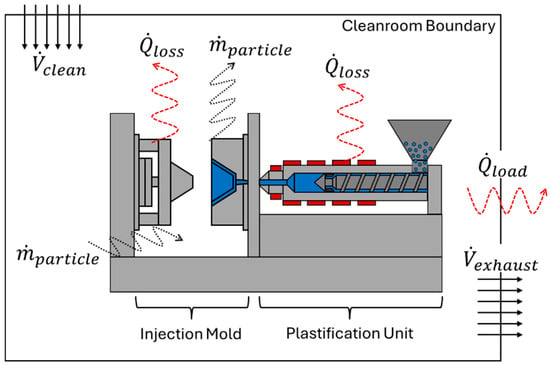
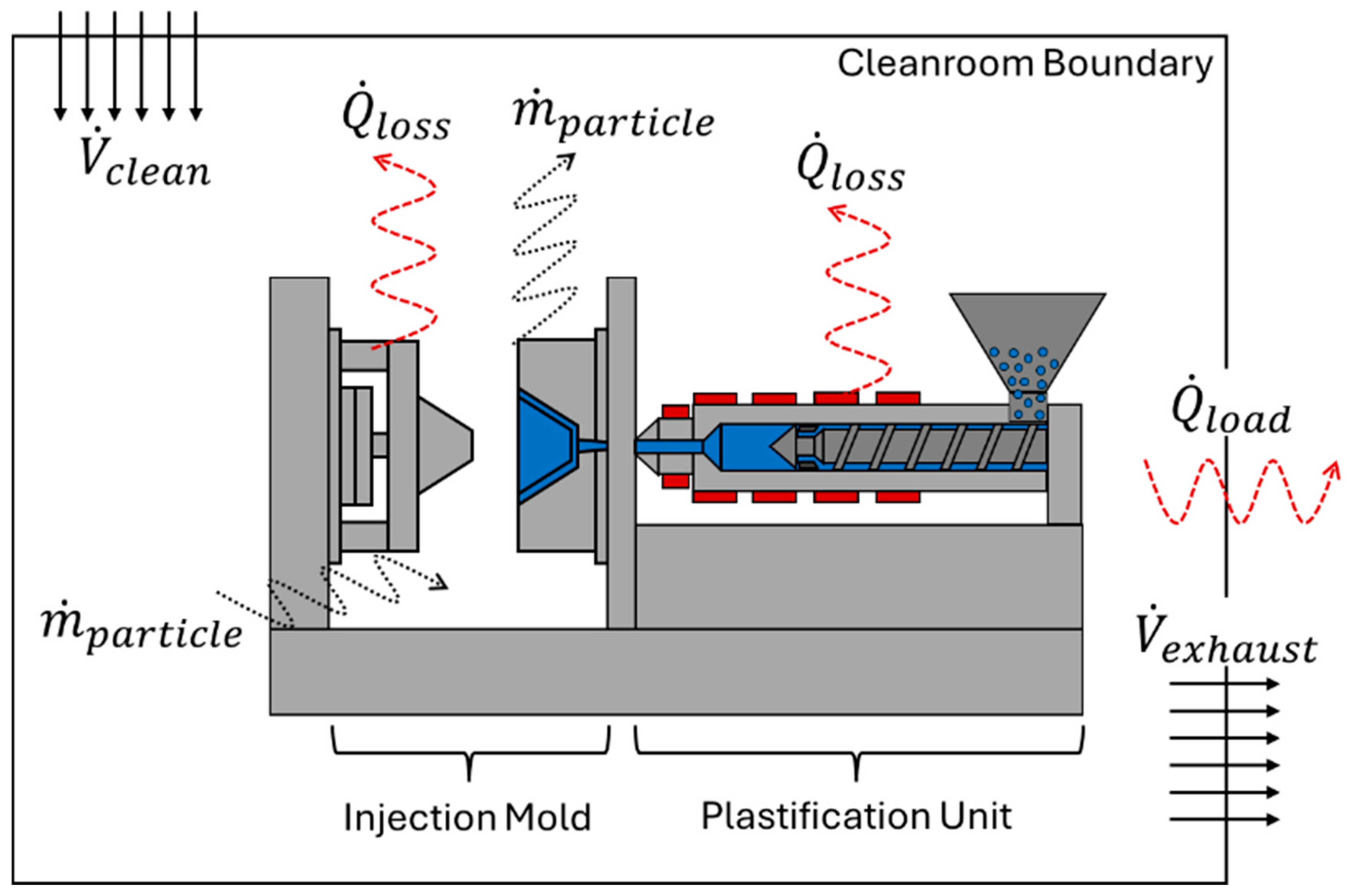
Integrating injection molding processes into cleanroom environments introduces several technical challenges (Figure 1). Injection molding machines generate significant heat through plastification processes, hot molds, and auxiliary equipment. Plastification temperatures up to 450 °C require mold set temperatures up to 180 °C [3], resulting in considerable thermal loads that must be removed by the cleanroom HVAC system. Accurate prediction of these heat loads is important for the design and operation of cleanroom ventilation systems, as oversizing HVAC systems leads to decreased energy efficiency [4]. Beyond their influence on the overall heat balance of the cleanroom, injection molding machines can also locally disturb the airflow. Heat released by the mold and machine surfaces generates buoyancy-driven plumes that interact with the airflow concept individually applied in cleanrooms. These thermal disturbances may alter local flow patterns around the mold and influence particle transport. As a result, particles generated within the machine or elsewhere in the cleanroom may be transported into the mold area where the polymer parts are produced, potentially increasing the risk of product contamination.
Figure 1.
Effects of an injection molding machine in a cleanroom.
Several studies have investigated injection molding in cleanrooms in numerous ways. A 1994 review of injection molding of medical parts emphasizes the complexity of handling injection molding processes in non-unidirectional cleanrooms of ISO class 8 [5] and the importance of controlling particles due to wear and personnel [6]. Injection molding in cleanrooms is typically conducted in environments corresponding to ISO class 7 or 8 [1]. Several integration concepts for incorporating injection molding machines into cleanrooms exist [7], and key parameters influencing the coupled thermo-fluid behavior include equipment and mold surface temperatures, machine layout, local airflow organization, ventilation configuration, and the use of localized control devices such as filter fan units (FFUs). The integration strategies include installing the complete injection molding machine inside the cleanroom, separating the plasticizing unit from the controlled area by a wall configuration, or placing the entire machine outside the cleanroom with a locally isolated mold region [1,7]. The highest cleanliness levels are achieved using isolator systems equipped with FFUs, enabling ISO class 5 conditions within the mold zone and supporting unidirectional airflow even when the surrounding cleanroom operates under non-unidirectional conditions [8]. For medical device production, EU-GMP Grade A conditions correspond to ISO Class 5, requiring strict control of airflow and contamination risk [9]. Accordingly, unidirectional airflow with a reference velocity of 0.45 m/s ± 20% is typically required in isolator-based systems [9]. For airflow design of unidirectional cleanrooms, simplified models of injection molding machines with constant surface temperatures and reduced geometries (e.g., cuboids) have been sufficient [2]. However, without considering thermal effects, particle emissions in the area of the mold and cavity were shown to increase with mold movement velocity [8]. Thermal influences have been addressed only partially: a critical mold temperature of 90 °C was identified, above which convective effects on the mold affected the unidirectional airflow [10].
High-temperature processes such as injection molding are therefore particularly critical under unidirectional airflow conditions, since buoyancy-driven convection may distort or oppose the imposed airflow direction, reducing flow uniformity and contamination control effectiveness [11]. This interaction between forced and natural convection is commonly characterized by the Archimedes number [12]. Early investigations have already demonstrated that thermal buoyancy can destabilize unidirectional airflow and lead to large-scale recirculation structures, with critical Archimedes numbers defining the limits of stable operation [13]. Another study further shows that even in simplified cleanroom configurations, buoyancy effects near heated equipment can induce stagnation zones and recirculation, significantly reducing ventilation efficiency and deviating from ideal plug-flow behavior [14]. During the design of supply air inlet configurations in non-unidirectional cleanrooms, the Archimedes number has also been used to describe the thermal plume from a cubic heat source [15]. Based on the Archimedes number, a design-oriented approach for unidirectional cleanrooms has been proposed, in which the supply air velocity is adjusted according to the thermal load of cylindrical heat sources to ensure flow stability. The study further introduces a stability criterion and quantifies the resulting contaminated volume forming around the heat source, enabling a load-dependent dimensioning of the airflow [11]. Without explicitly using the Archimedes number, the minimum air supply velocity to suppress convective effects originating from occupants has also been investigated [16]. The Archimedes number was further introduced to describe the airflow regime in isolated minienvironments with stationary heat sources [17].
Although several approaches exist to describe and control convective effects in cleanrooms, these concepts are based on simplified and stationary heat sources or occupants and are therefore not directly transferable to injection molding environments, where spatially distributed, process-dependent, and transient heat loads dominate in a partially open region with continuous exchange with the surrounding cleanroom. In general, particle contamination may originate from machine wear, the surrounding environment, or the polymer processing itself [18]. While isolators and localized airflow systems are widely used mitigation strategies, their effectiveness strongly depends on the coupled interaction between thermal loads and airflow organization. Nevertheless, despite previous investigations on individual aspects such as airflow configuration, thermal effects, and particle generation, a systematic understanding of their combined interaction in cleanroom injection molding remains insufficiently developed.
In addition to impacting airflow through convection, high-temperature applications increase the heat load on the cleanroom HVAC system. To ensure energy-efficient operation, it is therefore essential to design the HVAC system based on realistic heat load data. There are several approaches to determining the heat output of injection molding machines, but they differ considerably in scope and level of detail. Since the heat load cannot be measured directly, all approaches are based on some form of gross energy balance. Several studies use energy balances for injection molding but do not actually calculate the heat load for the cleanroom. Some studies present only simplified global balances without reporting individual heat flows [19,20]. Others restrict the analysis to single components such as the plasticizing unit and provide only phase-wise balance equations without numerical results [21]. One study focuses on internal energy conversion and a laboratory room balance, treating heat fluxes to the environment merely as residual boundary terms [22]. Studies that do estimate heat dissipation to the environment rely on strong simplifications and incomplete balances. One approach neglects the mold entirely, estimating surface losses from the plasticizing unit with fixed percentage assumptions, rather than measurements [23,24]. Another approach derives surface and drive losses from approximate convection/radiation models and constant manufacturer data. This results in a 24% discrepancy in the energy balance, which is attributed to uncertain cooling measurements [25]. Overall, none of these approaches provide a detailed, experimentally validated heat load for an injection molding production system under realistic cleanroom conditions.
Despite these advances, two key research gaps remain. First, there is no quantitative, measurement-based method that captures the total heat load of injection molding systems under realistic cleanroom operating conditions. Second, there is no universally applicable, dimensionless criterion to relate thermally induced convection to local particle contamination risk in the mold region. As a result, the coupled impact of thermal loads and airflow on contamination control remains difficult to assess and transfer across systems.
This study addresses these gaps on two levels: First, the total heat load introduced into the cleanroom by the injection molding process is quantified by considering the machine, mold, temperature-control unit, automation, and produced parts under realistic operating conditions. Second, the resulting convection effects due to the injection molding machine’s high surface temperature in the cleanroom are examined, focusing on the critical region around the mold where elevated surface temperatures can disturb the downward airflow in the cleanroom, resulting in unknown contamination risk.
We therefore propose and apply a simple, measurement-based procedure to quantify the heat load of injection molding machines in cleanrooms, considering the heat load introduced by the injection molding process. This procedure is based on an energy balance that includes the injection molding machine, temperature control unit, mold, automation, and produced part. This procedure enables us to distinguish between the machine’s process-independent heat load and process-dependent heat load, which mainly originate from the mold and peripheral devices. Thus, it provides quantitative input for HVAC design and cleanroom energy assessments. On a local scale, we examine how these thermal loads manifest as flow structures and potential sources of particle contamination in the mold area. We describe the mixed convection around the mold analytically using the Archimedes number. Experiments combining Schlieren flow visualization and particle counting link the particle load in the mold area to the Archimedes number. This allows for assessment of contamination risk under different operating conditions, as required by EU regulatory standards for medical production [9]. These experiments also assess the effectiveness of filter-fan units in suppressing convective plumes. The results contribute to a better understanding of the interaction between manufacturing processes and cleanroom airflow and provide guidance for the design and operation of injection molding production in controlled environments.
2. Materials and Method
2.1. Heat Load from Injection Molding into Cleanroom Environment
2.1.1. Gross Energy Balance of Production Cell
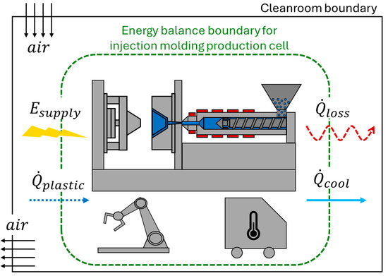
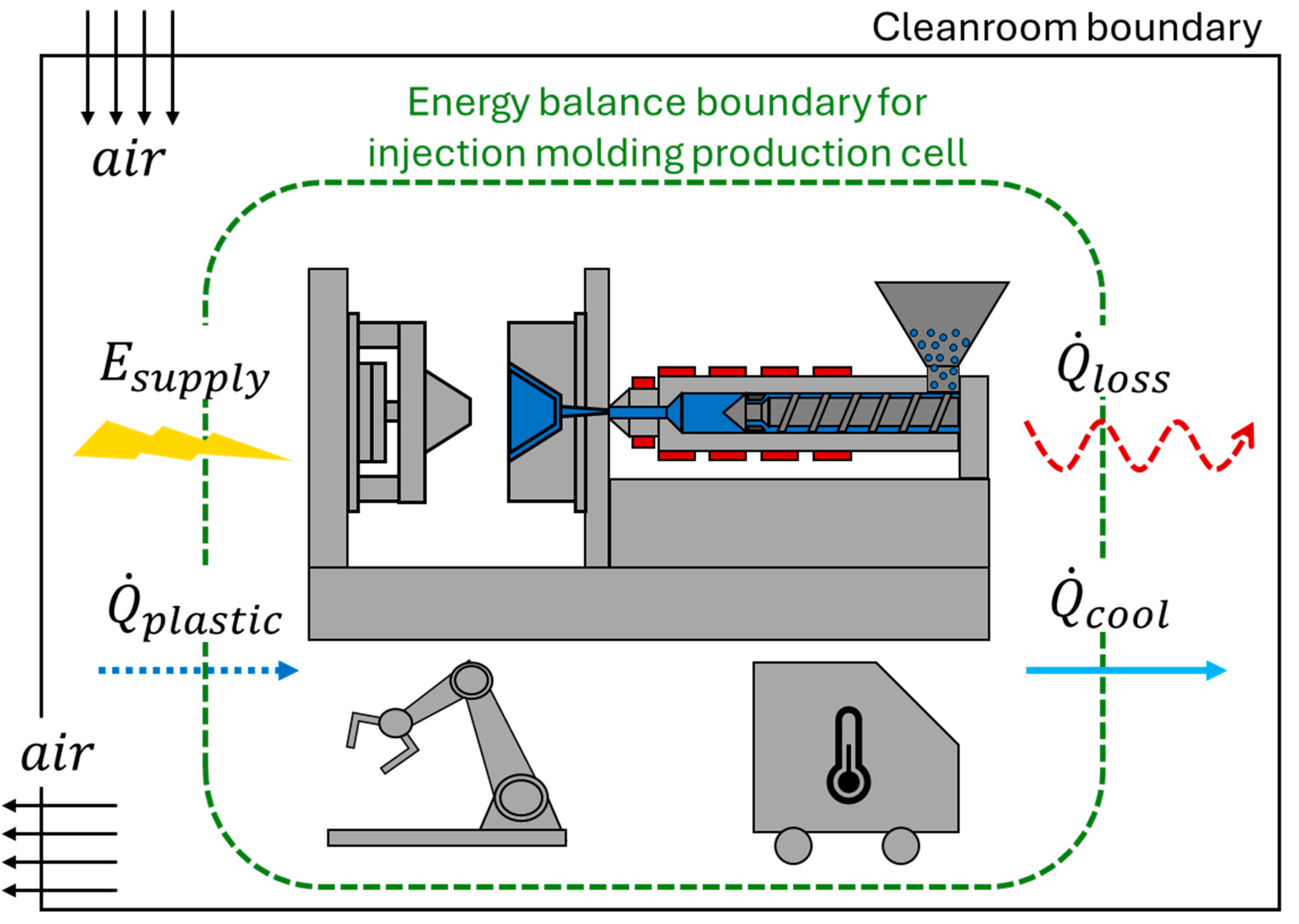
Heat loads from injection molding production cells inside cleanrooms must be discharged by the air conditioning system as heat loads. This heat load cannot be measured directly. Therefore, we calculate the energy balance of the injection molding production cell, which includes the injection molding machine, automation system (e.g., unloading robot), temperature control unit, injection mold, and produced part (compare Figure 2). The produced part will remain in the cleanroom for further processing (e.g., packaging or sterilization) until it cools to the surrounding temperature. All cables and hoses within the defined energy balance boundaries are included. The necessary supply connections for injection molding production cells include an electric connection, cooling water, and a mass flow of plastic granulate into the injection molding machine. Three energy flows can be derived from these supply connections: work in the form of electricity, heat stored in the cooling water, and heat stored in the plastic granulate. Within the energy balance boundaries, electrical energy is converted into movement (e.g., opening and closing the mold and moving the automation system) and heat (e.g., hot runner and cylinder heating). Through movement and heating, energy dissipates into the cleanroom. Additionally, the produced part is ejected from the injection mold before reaching the surrounding air temperature. Therefore, if the produced part remains in the cleanroom, it dissipates heat into the cleanroom. Since this heat load cannot be measured directly, an energy balance defined by the first law of thermodynamics is derived.
Figure 2.
Gross energy balance for an injection molding production cell, including the injection molding machine, the mold, the temperature control unit, and automation systems (e.g., robots). The produced part stays within the energy balance boundary until it is cooled to the surrounding temperature.
In words: the change in a system’s internal energy is equal to the sum of the work and heat applied to or generated by the system. For the injection molding production cell, the corresponding energies are the electrical consumption , the heat through the mass flow of plastic granules , the heat in the cooling water and the heat load . Applying this to the first law of thermodynamics yields
Assuming steady-state operation, we can set :
Except for the heat load , all energy flows can be measured directly. For a steady state, the heat load can thus be determined as
2.1.2. Gross Energy Balance of Injection Molding Machine
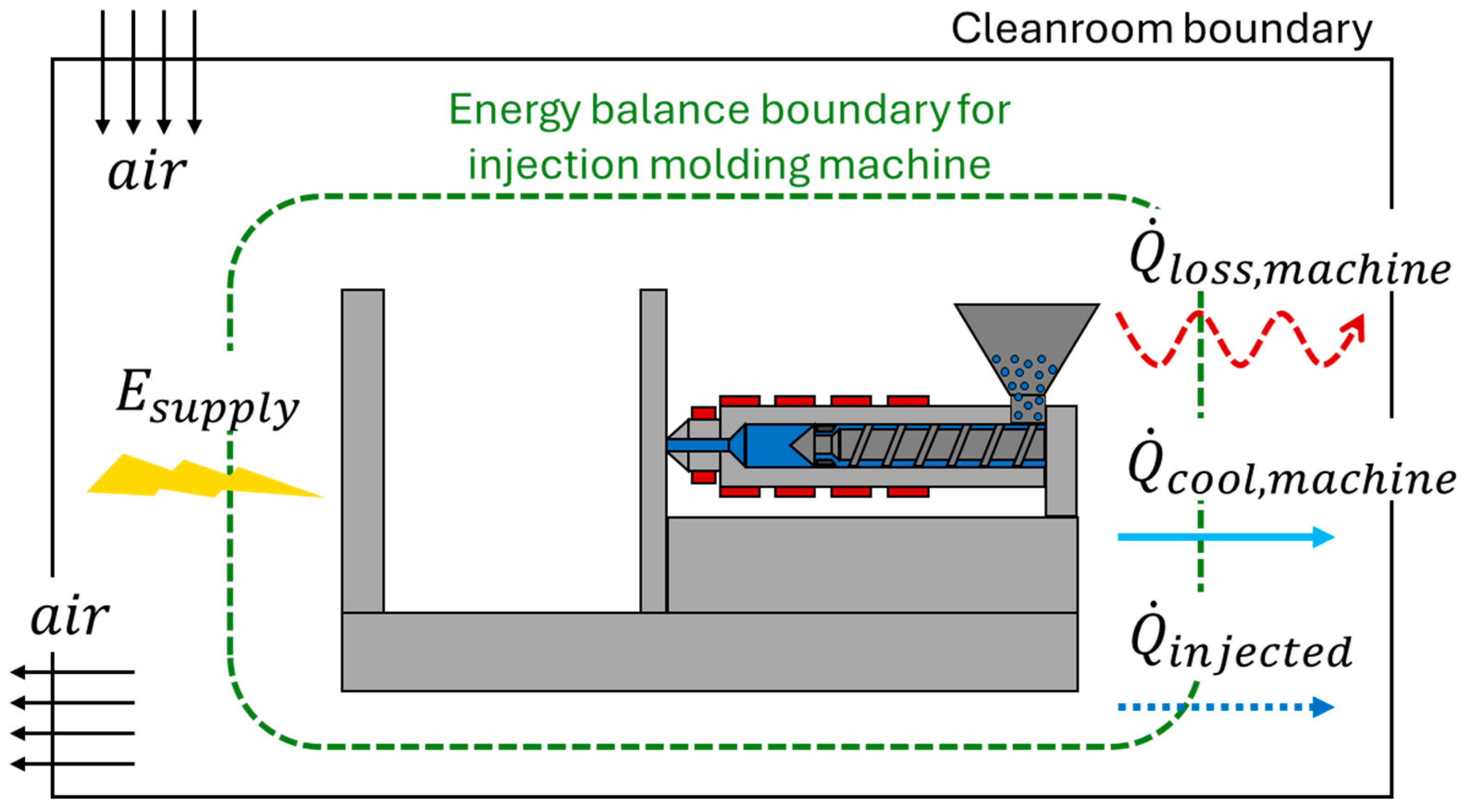
Since the peripheral devices are variable, the injection molding machine is additionally analyzed in isolation (i.e., excluding the peripheral devices from the energy balance). The energy balance boundaries for the injection molding machine include only the machine itself. The automation system, temperature control unit, cables, hoses, and the produced part are not included (see Figure 3). Energy flows can be derived from the supply connections (Figure 2 in Section 2.1.1). Electrical energy is supplied to the machine via the power supply. Part of the machine’s heat losses are discharged via the machine cooling . During the process, the metered plastic is heated and melted in the plasticizing unit and then injected into the mold under high pressure (two thousand bar or more). Thus, the plastic acts as a heat sink for the energy balance. To distinguish this heat sink from the heat source in the energy balance of the entire production cell, it is referred to as . The remainder is the heat lost to the environment , either by convection, radiation, or dissipation. Under steady-state conditions, the gross energy balance can be stated as follows:
Figure 3.
Energy balance of an injection molding machine without peripheral devices or a mold.
The energy consumption of the injection molding machine and the cooling via the process water can be determined by measurement. However, the heat content of the plastic, on the other hand, cannot be measured directly during operation. It can be determined using the thermal characteristics of the plastic and the mass of processed plastic . Differential scanning calorimetry (DSC) can be used to determine the temperature-dependent enthalpy change of the plastic. Given the temperature of the plastic when it is fed into the plastification cylinder and the melt temperature when it is injected into the mold (approximated by the set temperature at the injection nozzle), the heat discharged by the injected plastic can be calculated. Note that the melt temperature deviates from the set nozzle temperature and changes during injection with the injection stroke. This issue has been discussed in various studies, but no simple, accurate method has been proposed to estimate the melt temperature. One approach uses artificial neural networks for this estimation [26,27]. However, for the energy balance, this assumption proved sufficient.
2.1.3. Experimental Setup Heat Load
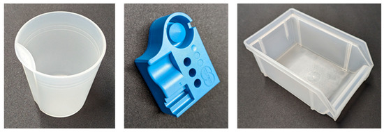
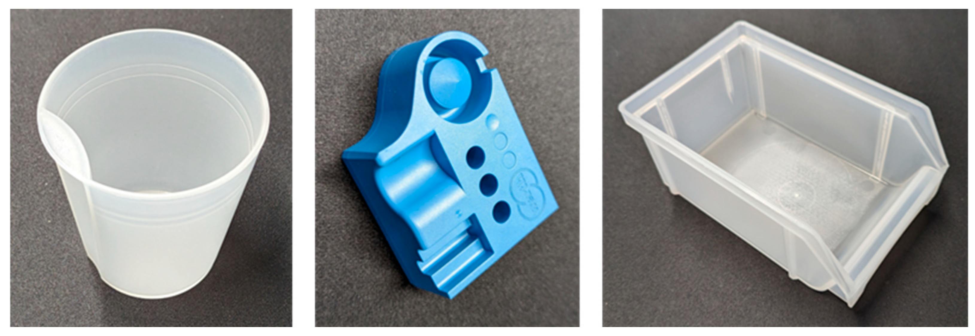
It is crucial to apply the previously proposed gross energy balances for the injection molding machine and the complete production cell under steady state conditions. To ensure that the steady state has been reached, the measurements begin as soon as the surface temperatures of the mold and plastification cylinder are balanced with the surroundings, meaning that they remain constant throughout the process (i.e., they diverge around a mean value with a maximum difference of 0.5 K). To compare measurements taken with different machine settings, the energy is derived over time to determine the mean heat loss in power for different processes: . This time-dependent comparison also allows for different production and measurement times for each machine/mold combination. Measurements are taken on two injection molding machines: a fully electric machine with one hundred tons of closing force (manufactured in 2023) and a hydraulic machine with 80 tons of closing force (manufactured in 2016). Three molds will be used (see Figure 4): (i) a cup with a capacity of 0.25 liters made of polypropylene (PP) with a mass of 45 g and used on both machines; (ii) a complex geometry specimen made of polyphenylene sulfide reinforced with glass fibers (PPS GFR) with a mass of 59 g and used only on the hydraulic machine; (iii) and a box with dimensions of 160 × 100 × 75 mm made of PP with a mass of 110 g and used only on the electrical machine. Due to size limitations, not all molds were used on botch machines. An overview of the mold-machine combinations and test parameters is given in Table 1.
Figure 4.
Produced parts. (Left): A cup made of PP (45 g). (Middle): A test specimen made of PPS (59 g). (Right): A box made of PP (110 g).
Table 1.
Overview of experimental cases for determining the head load of the injection molding production cell.
The thermal characteristics of each material are determined by DSC measurement, as described in Appendix A. The electrical power consumption of the machine was measured at five locations: (i) the main power supply, (ii) the drive system, (iii) the heating bands of the cylinder, (iv) the hot runner system, and (v) the power connectors for external devices. Subtracting the measurements from (ii) to (v) from the main power supply (i) determines the energy consumption of the machine’s control system. Power is determined at each measurement point by local current measurement with cable conversion current transformers for each phase. Voltage is only measured at the supply connector for each phase and is considered constant throughout all measurement points. For the heat flow represented by the cooling water, the flow rate, as well as the forward and reverse flow temperatures, are measured. Additionally, the surface temperatures of the mold and plastification cylinder are measured. The sensors used for flow rate and temperature are ultrasonic flowmeters, resistance thermometers (PT1000), and thermocouples (type J). Electrical power is measured at 10 ms intervals to capture all load peaks during the process. The ultrasonic flowmeters have a response time of 1000 ms, which is used as the measurement interval for flow temperatures. Since the surface temperature changes more slowly than the previous measurement points, those were measured at 5000 ms intervals. A Beckhoff SPS system was used to achieve the low measurement interval of the power measurement.
2.1.4. Uncertainty Analysis
This chapter discusses how measurement uncertainties affect our estimates for the individual gross energy balances. In what follows, the measurement uncertainty is determined using the Gaussian error propagation law. For the electrical power consumption, the power is determined from the measured voltage and current. Based on the sensor specifications, the following uncertainties are applied: voltage measurement (Beckhoff EL3403, Beckhoff Automation GmbH & Co. KG, Verl, Germany) ± 0.5% and current measurement (Wago split-core current transformer, accuracy class 1, WAGO GmbH & Co. KG, Minden, Germany) ± 3% combined with the measurement terminal (Beckhoff EL3403) ± 0.5%. Using Gaussian error propagation, the relative uncertainty of the power is 3.54%.
For the energy flows based on the plastic mass flow (i.e., plastic fed to the machine, plastic injected into the mold and plastic ejected from the mold), the total mass is determined by the number of parts produced and the weight per part. The weight per part is measured with a linear deviation of ±0.2 g, while the specific enthalpy is derived from DSC measurements and temperature estimates. The DSC instrument (Mettler Toledo DSC 3+, Mettler-Toledo GmbH, Gießen, Germany) itself exhibits a calorimetric precision of approximately 1% and a systematic deviation of up to 2.5% according to manufacturer specifications. However, for polymer measurements, additional uncertainties arise from baseline determination, peak integration, and the transfer of laboratory measurements to process conditions. For each plastic processed, three samples were measured with a maximum deviation of 1.6%. An additional limitation arises from the indirect estimation of melt temperature, which is based on the nozzle set temperature, rather than direct measurement. This assumption introduces an additional systematic uncertainty. Therefore, a conservative overall uncertainty of 15% is assumed for the plastic energy flows.
The thermal power of cooling channels is calculated from the mass flow and temperature difference in the fluid via heat meters. For the mass flow, vortex flow meters (Huba Control 230, Huba Control AG, Walddorfhäslach, Germany) are used with an uncertainty of , according to manufacturer data sheets. The temperature is measured with an integrated PT1000 resistance thermometer in the supply and return mass flows with an uncertainty of . With a typical mass flow of 5 L/min and a temperature spread of 5 K, this yields a relative uncertainty of 30.7%. Due to the relatively low mass flow compared to the sensors’ range of the measurement (1.8 to 150 L/min) the uncertainty of the mass flow can be considered the most critical influence.
Overall, the uncertainty analysis shows that the electrical power can be determined with comparatively low uncertainty (~3.5%), while the plastic energy contribution is associated with moderate uncertainty (~15%), primarily due to the indirect estimation of melt temperature. The highest uncertainty arises from the heat flow measurements (~30%), dominated by the limited accuracy of the mass flow sensors at low flow rates. The energy balance is evaluated over extended production periods (approximately 1 h), using time-integrated quantities (kWh). Therefore, differences in temporal resolution between measurement systems have a negligible impact on the averaged results, as transient fluctuations are inherently smoothed out. Since all measurement data are acquired within a single system (i.e., a Beckhoff PLC TwinCat 3), temporal misalignment of measurement signals is minimized. These effects are considered secondary compared to the dominant measurement uncertainties discussed above. Consequently, the reported heat loads and derived quantities should be interpreted as robust trends, with the main relative uncertainty in the order of 40%.
2.2. Flow Analysis Inside the Injection Molding Machine
2.2.1. Analytical Description with Dimensionless Numbers
In addition to the effects on HVAC systems of cleanrooms, the heat load caused by injection molding processes affects the airflow regimes. Convective effects, especially around the injection mold and the plastification unit, form buoyancy plumes influencing the cleanroom flow regime in an unknown manner. Since the part produced within the isolated mold region is the most critical aspect of injection molding in cleanrooms, it is crucial to understand the flow effects around the mold in detail to produce contaminant-free parts. Effects of buoyancy plumes around the plastification unit are not part of this study. Consequently, high-temperature applications such as injection molding are considered critical in cleanrooms.
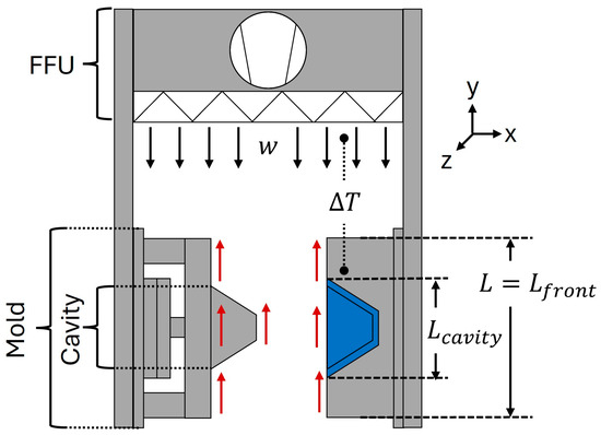
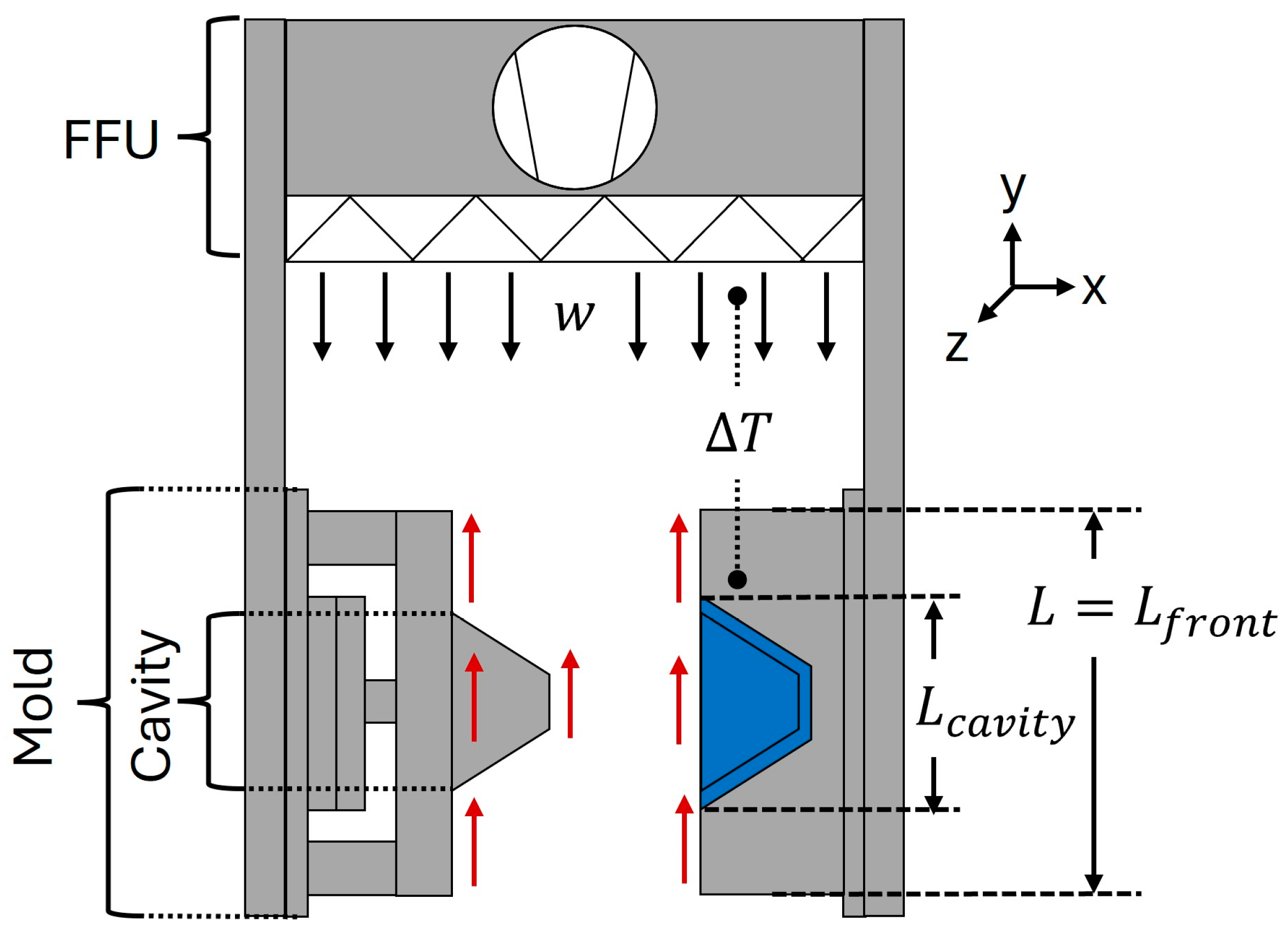
The flow in the injection mold area can be described as opposing mixed convection: a forced flow from the filter fan unit (FFU), opposed by natural convection on the mold’s surface (Figure 5) [28]. This kind of flow is generally described by quantifying the magnitude of buoyancy forces relative to forced convection forces and is typically expressed as the Archimedes number () [12]:
with the characteristic length , the gravitational constant , the thermal expansion coefficient of air , the temperature difference between the fluid and the wall and the velocity of the forced airflow . The driving force is generally said to be forced convection when the Archimedes number is small, and natural convection can be neglected. When the Archimedes number is large, the opposite is true. Consequently, critical Archimedes numbers describing the transition from forced to free convection have been investigated in several studies from general and specific perspectives, including cleanroom applications. For vertically heated surfaces, the critical Archimedes number under which natural convection can be neglected varies between 0.3 [29] and 0.225 [30]. In other works, fully forced flows are generally described for [31] and [32]. For cleanrooms, the critical Archimedes number to ensure that the airflow is unaffected by convective effects ranges from [17] over [15] and [13] to [14]. In this approach, the Archimedes number is linked to the overall cleanroom temperature rise and the source is represented by an equivalent cylinder. However, because the method considers the temperature change in the entire cleanroom flow, it cannot be applied directly to localized heat sources such as injection molds.
Figure 5.
Airflow within the mold area of an injection molding machine. There is forced flow from the top by the FFU, as well as free convection on the mold surface.
As is common in the literature [33,34], the temperature difference can be expressed as the convective wall heat flow as
Here, is the convective surface area, is the temperature difference between the fluid and the wall, is the Nusselt number, is the thermal conductivity of the surrounding air and is the characteristic length. Inserting it into Equation (6) yields the following Archimedes number:
The characteristic length is defined as the length of the convective surface in the direction of the flow and equals the height of the injection mold (y-direction in Figure 5). The area is the projected front surface of each mold half. Given the mold depth (z-direction in Figure 5) and height (y-direction in Figure 5), the area can be determined as . The shape of the mold can be characterized via the following geometric simplex:
Due to the inhomogeneous surface temperature and the complex geometry, it is difficult to model or measure the mold’s heat load via convection to the environment. Because the exact surface temperature distribution depends on the mold design (e.g., cooling channels and mold insulation), it cannot be generalized. However, two idealized conclusions can be drawn: (i) The cavity is the hottest part with a constant temperature equal to the set temperature of the temperature control unit. (ii) The front of the mold has a decreasing temperature, from the cavity temperature to the surrounding temperature. Based on these conclusions, only the front surface of the tool is considered for convection. This is where the cavity is located and therefore the highest surface temperatures occur. The temperature can be considered constant on cavity surfaces (an ideal cavity would have a constant surface temperature equal to the set flow temperature). The temperature of the remaining mold front surface decreases with increasing distance from the cavity. Thus, the heat dissipation of the mold can be divided into two sub-areas: the cavity and the mold front:
Since the surface of the cavity lies in the center of the mold front surface, both regions are exposed to the same global mixed convection flow field imposed by the FFU and buoyancy interaction. Therefore, the Nusselt numbers are not treated as independent local quantities, but as part of a coupled flow regime and are therefore assumed equal in both equations: . The assumption therefore does not imply identical local heat transfer conditions but rather represents a single effective Nusselt number describing the overall flow regime. To assess the sensitivity of this assumption, a ratio is introduced, allowing deviations between both regions to be considered. The total heat dissipation can then be expressed as
This leads to a linear dependence of the Archimedes number on the scaling parameter . Variations in therefore result in a proportional scaling of the Archimedes number without altering its functional structure or the resulting flow regime classification. Although the Nusselt number cancels out in the final formulation (Equation (18)), this intermediate analysis shows that deviations between local heat transfer conditions only affect the result through a linear weighting of geometric contributions.
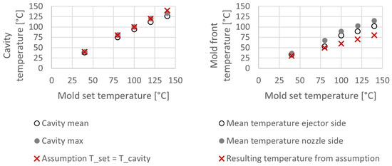
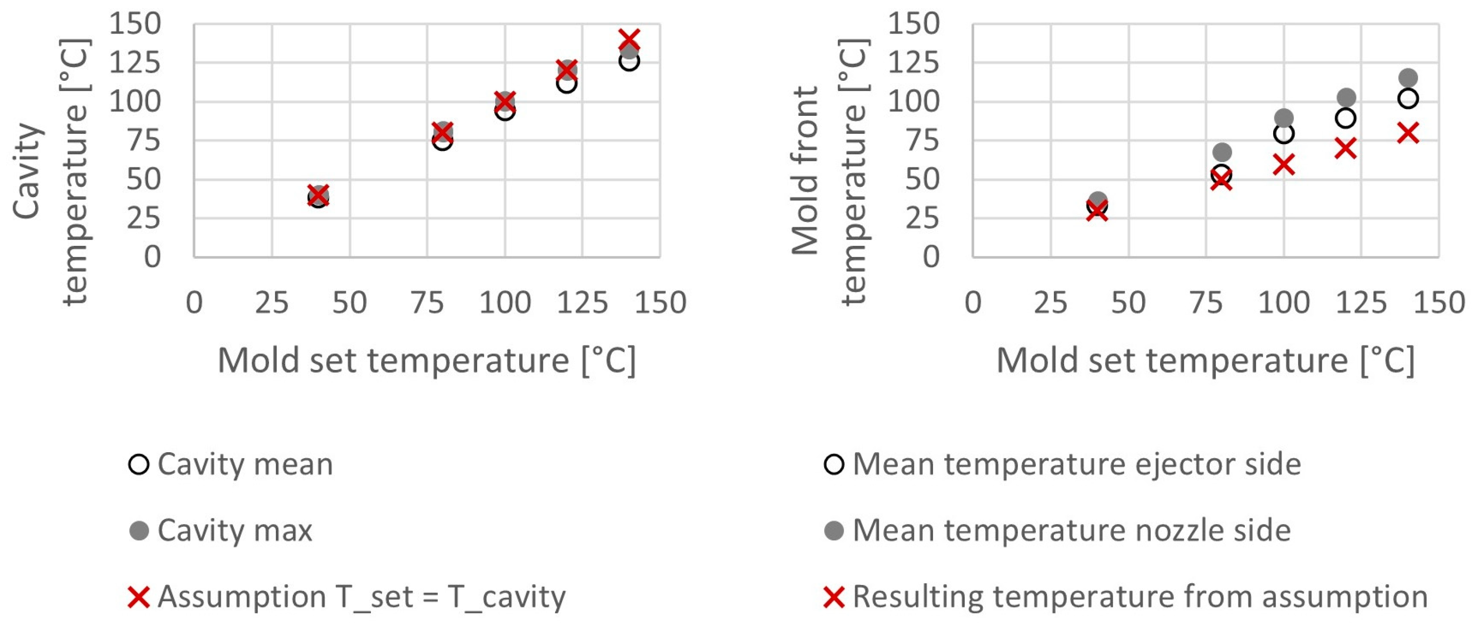
Assuming the surface temperature of the cavity is equal to the set temperature of the temperature control unit, () represents an ideal mold. Comparison of the assumption with infrared imaging shows that with an increasing set temperature, the introduced uncertainty increases (Figure 6 left). The mean front temperature of the mold depends on the cooling channel design, insulation, and local heat transfer conditions, and exhibits an inhomogeneous distribution with a decreasing gradient from the cavity toward the mold edges. To obtain a practical formulation, the front temperature is approximated as the average of the air temperature and the set temperature of the temperature control unit , yielding . Infrared measurements of the mold surface (Figure 6 right) show that this assumption slightly underestimates the actual mean surface temperature. A more accurate representation could be obtained using an area-weighted temperature; however, this would significantly increase model complexity. The underestimation of the front temperature leads to a reduced predicted heat flux, which partially compensates for the expected overestimation of the Nusselt number (and therefore an increased predicted heat flux) on the cavity surface. As a result, the combined effect of both assumptions remains within a consistent order of magnitude. Substituting (11) and (12) into (10) with the described simplifications yields
Figure 6.
(Left): Cavity mean and maximum temperature from infrared imaging over the mold set temperature. (Right): Mean mold front temperature from infrared imaging over the mold set temperature.
The final term is extracted and defined as the characteristic convection length , which depends on the mold size and cavity shape:
This geometric simplification of representing the mold by a cavity and a front surface to length in flow direction is reflected in the definition of the characteristic convection length, which aggregates the contributions of both regions. Variations in cavity size or mold geometry therefore influence the Archimedes number through linear scaling, while preserving the general formulation. Substituting (9) and (14) with the characteristic convection length from (15) into the Archimedes number (8) yields
Since the Nusselt number and the thermal conductivity are for the same flow condition and the surrounding air, respectively, they cancel out. Additionally, a dimensionless temperature difference can be defined as follows:
This results in the following expression for the Archimedes number:
The introduced assumptions (uniform Nusselt number, simplified temperature distribution, and reduced geometry) represent first-order approximations to enable an analytical description of the system. Their impact on the resulting formulation is limited: the Nusselt number cancels out in the final expression for the Archimedes number, reducing sensitivity to local heat transfer variations. The assumed front temperature corresponds to a linearized temperature profile, which is supported by infrared measurements showing a monotonic decrease from cavity to mold edge. Variations in this assumption primarily affect the magnitude of the heat flux but do not change the qualitative flow regime classification. Similarly, the geometric simplification captures the dominant heat-emitting surfaces while neglecting secondary features that mainly influence local flow structures. Consequently, the introduced assumptions can be interpreted as first-order approximations that enable a physically consistent scaling description of the flow, rather than a detailed representation of local heat transfer phenomena.
2.2.2. Analysis Buoyancy-Driven Flow near the Injection Mold
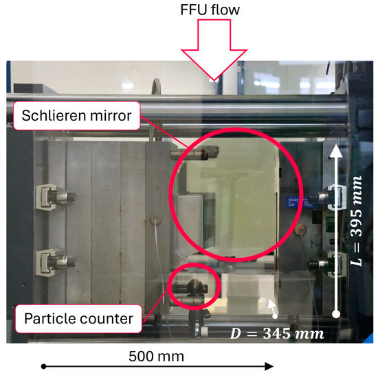
Experiments with the box-mold from the heat load measurement (Section 2.1.1) were conducted to analyze the flow regime for different mold set temperature and FFU velocity combinations (i.e., different Archimedes numbers). To achieve this, flow visualization using Schlieren photography was conducted. This enables linking the flow visualization to the analytical flow description from Section 2.2.1. Schlieren photography was chosen as the tool to visualize the airflow over classical fog visualization, as it provides a highly sensitive and completely non-intrusive visualization of convective airflows, and it has been successfully applied to cleanroom flows in former studies [35]. In addition to the flow visualization, the experiments analyze the dependency of the particle load within the mold area on the established dimensionless Archimedes number. Therefore, a particle counter was placed 100 mm beneath the outer edge of the cavity and 50 mm in front of the mold’s front surface. The particle counter is oriented horizontally with the opening facing towards the discharge side of the injection molding machine. An overview of the experimental setup with the exact placing of the particle counter sampler and the exact region of schlieren photography is provided in Figure 7, together with the mold dimensions for the calculation of the Archimedes number. Inserting the constant values into Equation (18) results in the case-dependent Archimedes number:
Figure 7.
Experimental setup for measuring FFU volume flow , supply-air temperature and particle load. Aerosol is injected from within the drop shaft (not pictured). The red circle indicates the region captured by schlieren photography.
Leaving the mold set temperature, cleanroom air temperature and the FFU flow velocity together with the particle load as measurement parameters. To determine the mean forced airflow velocity from the FFU, the airflow volume was measured at the FFU’s suction inlet with a volume flow hood. The volume flow hood also measures the supply air temperature which equals the cleanroom air temperature. Additional to the mold set temperature at the temperature control unit, the mold’s surface temperature was measured using an infrared camera. The particle counter sampler beneath the mold cavity is oriented with the probe facing toward the cavity. The aerosol injection point was chosen within the drop shaft, based on preliminary tests. The injection within the drop shaft ensures enough particles to conclude significant findings. The aerosol generator used is a Topas ATM 228 (Topas GmbH, Dresden, Germany) with DEHS (density: 910 kg/m3, Topas GmbH) as aerosol liquid and a Solair 3100 (Lighthouse Worldwide Solutions, White City, OR, USA) particle counter. Particles are generated and counted in relevant cleanroom class sizes, ranging from 0.3 µm to 25 µm. Measurements were taken at different mold set temperatures ranging from 20 °C to 140 °C in 20 °C increments, at different FFU velocities (0.22 m/s, 0.34 m/s, 0.50 m/s, 0.67 m/s, and 0.89 m/s), and at different mold stroke widths (10 mm, 15 mm, 23 mm, and 35 mm). Additionally, videos were produced using Schlieren photography to enable visual flow analysis during the measurements (see Supplementary Materials).
3. Results and Discussion
3.1. Heat Load of Injection Molding Production Cells
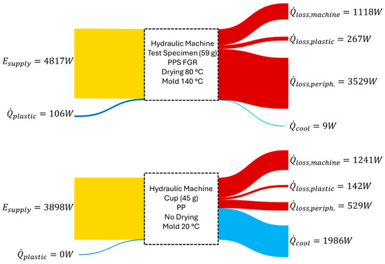
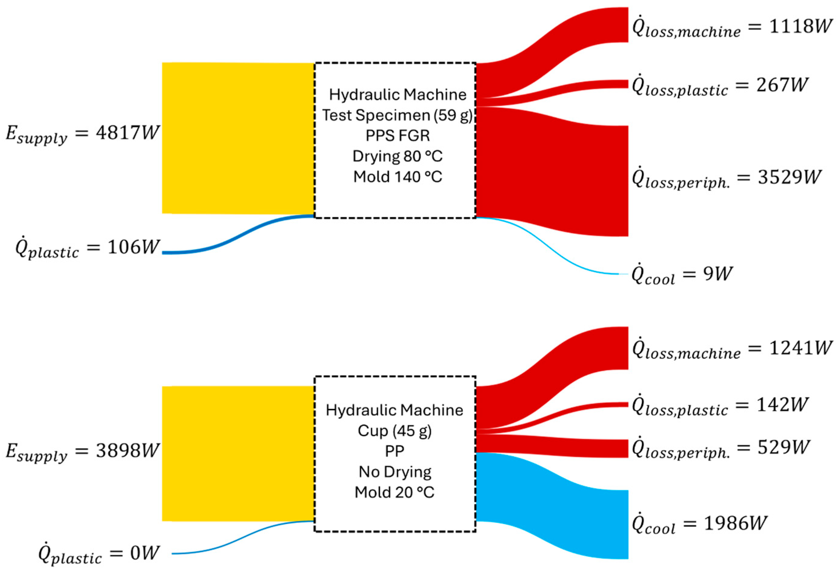
The results for the energy balance of the hydraulic machine are shown in Figure 8. The production of the test specimen was the only instance in which the plastic was dried prior to production. In all other cases, it was stored in the cleanroom prior to production to reach ambient temperature. Therefore, an energy supply flow for the plastic is only available for the test specimen made from PPS GFR. To produce the test specimen, the injection molding machine and the peripheral devices required nearly no water cooling. Almost all electrical energy consumption and the heat in the dried plastic result in additional heat load into the cleanroom of 4.9 kW. Due to the high mold set temperature, the temperature control unit constantly heated the mold to counteract heat loss to the surroundings while cooling the plastic part. The peripheral devices contributed most to the heat loss due to the relatively high mold temperature of 140 °C. The cup production process on the same machine required less energy. Unlike the test specimen, where cooling the machine and TCU was unnecessary, the mold for the cup must be cooled to 20 °C. This is evident in the 2 kW cooling water stream. Similarly, the heat loss of the peripheral devices decreased significantly due to the lower mold temperatures (0.5 kW vs. 3.5 kW). However, the power consumption of the injection molding machine increases by 0.6 kW (i.e., 30%). This increase is attributed to the cup’s shorter cycle time (60 seconds vs. 34 seconds) and the associated more frequent machine movements per unit of time. Nevertheless, the heat load from the injection molding machine remains approximately constant (1.1 kW and 1.2 kW) across both processes. The heat loads of both injection molding machines are significantly lower than their maximum connection power. The connection power of 117 kW for the hydraulic machine resulted in a 1.1 kW heat load, whereas the electrical machines’ connection power of 47 kW resulted in a 2.1 kW heat load. These comparatively high connection powers arise from two factors. First, higher power is required during preheating than during steady production, when only temperature maintenance is necessary. Second, the required connection power additionally reflects the available power connectors for peripheral devices on the machine.
Figure 8.
Results of the energy balance and heat loss of a hydraulic injection molding machine.
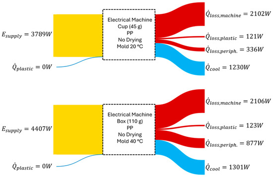
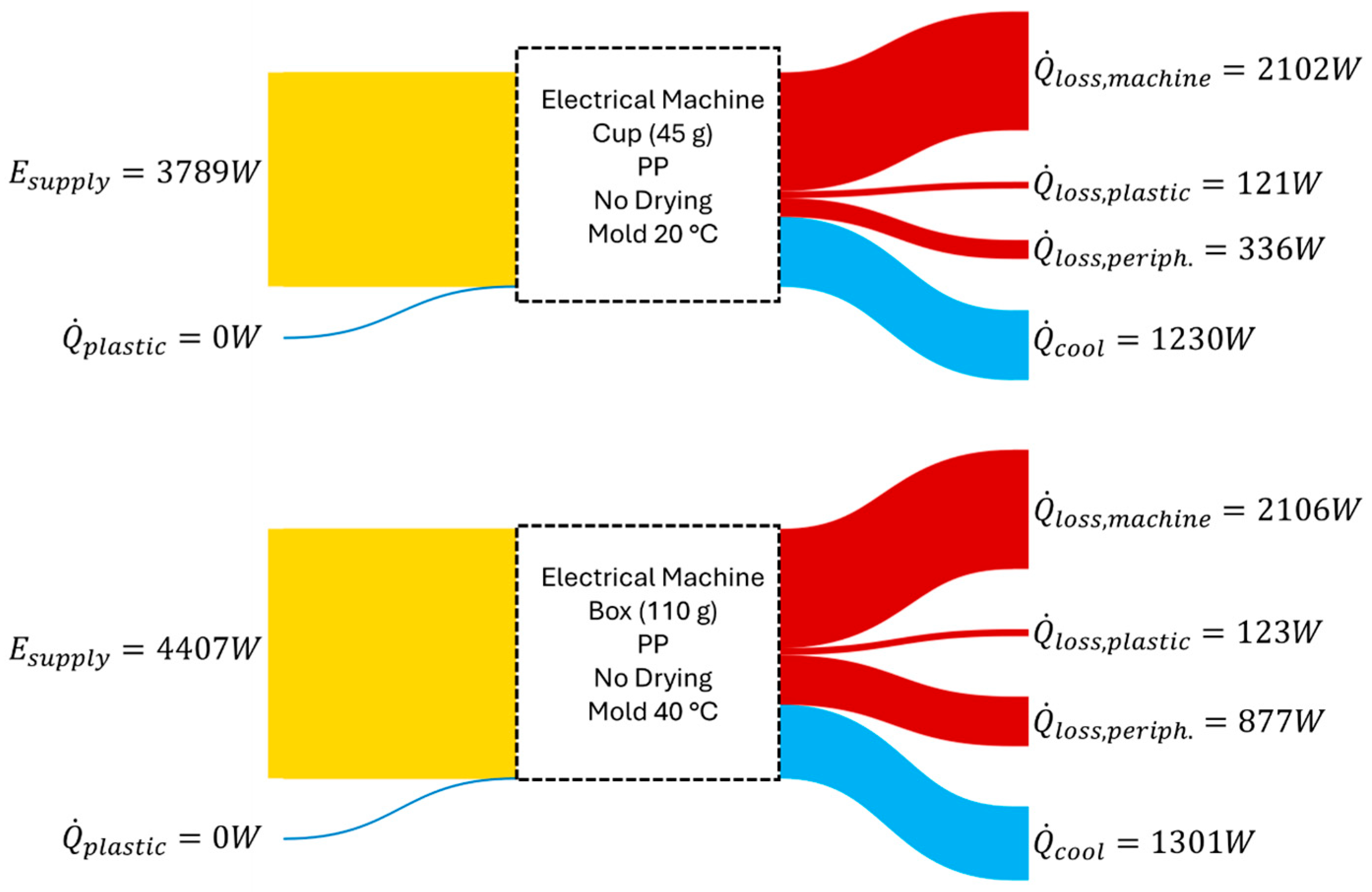
Similar investigations can be observed for the electric machine (Figure 9). Since both components of the electric machine are made of PP, the processes are more similar than those on the hydraulic machine. The plastic was not preconditioned, so the energy flow supplied to the injection molding production cell by plastic is zero. Due to the low mold temperatures of 20 °C and 40 °C, heat losses from the periphery are not significant. The box’s higher energy consumption compared to the cup can be attributed to its double material throughput (4.1 kg/h vs. 7.7 kg/h). Again, the heat load from the injection molding machine remains constant at 2.1 kW regardless of the process. Due to the larger mold for the box and the higher mold temperature, the heat load from the peripherals also increases compared to the cup. When comparing the cup on the electrical and hydraulic machines, it is evident that the energy consumption is similar (3.8 kW vs. 3.9 kW). This differs from trends reported in the literature: that electric machines operate more efficiently [36,37,38,39]. However, differences in machine generation and operating conditions are not consistently reported in the cited studies. Injection molding machine manufacturers claim in non-scientific publications that modern servo-hydraulic machines can be less energy-demanding than fully electrical machines [40]. However, the heat losses from the injection molding machine differ, at 2.1 kW for the electrical machine and 1.2 kW for the hydraulic machine.
Figure 9.
Results of the energy balance and heat loss of an electrical injection molding machine.
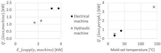
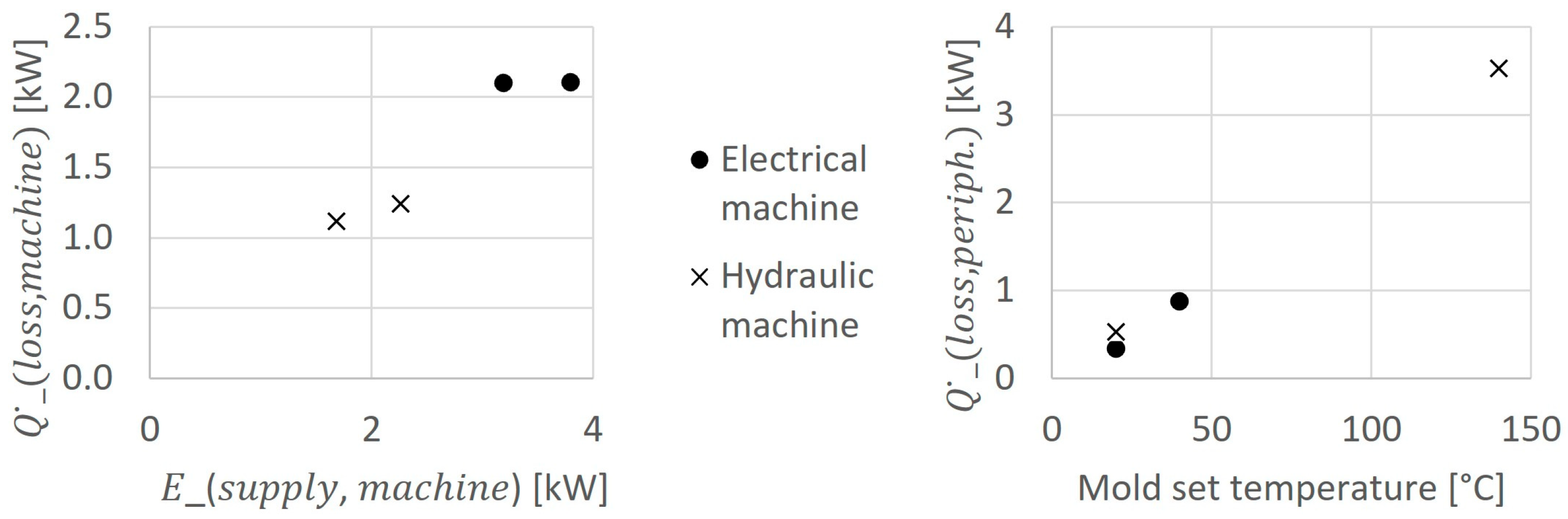
The significant variation in heat load between the two molds on the hydraulic machine in the clean room illustrates the difficulty plant engineers face in quantifying heat loads during the planning phase. In this case, the overall heat loads differ by 2.5 kW, while the heat loss of the injection molding machine remains constant. This suggests that heat load from the injection molding machine depends less on the process than heat load from the peripherals. These two dependencies are examined in detail (compare Figure 10). The injection molding machine’s heat load is considered in relation to its power consumption. The diagram shows that there is only a slight correlation between the machine’s heat load and the process, though the heat load of the electrical machine is higher. To examine the influence of the process on the heat load of peripheral devices, the mold temperature is considered. This indicates a linear relationship: as the mold temperature rises, the heat load from the peripherals, including the mold, increases. The variables related to the process are the mold temperature and size, as well as the temperature control unit and plastic throughput.
Figure 10.
(Left): Heat load of the injection molding machine dependent on power consumption. (Right): Heat load of the complete production system (including all peripheral devices and the mold), depending on the mold set temperature.
In industrial HVAC design practice, the thermal load of injection molding machines is often approximated using a fraction of the installed electrical power as a conservative estimate. The present results show that the measured heat load released to the surrounding environment is substantially lower than the installed electrical power (117 kW for the hydraulic machine and 47 kW for the electric machine). This suggests that such design approaches may lead to an overestimation of the heat load of injection molding systems. This comparison provides a reference to common engineering practice and highlights the added value of the measurement-based approach proposed in this study.
3.2. Airflow Inside the Injection Molding Machine
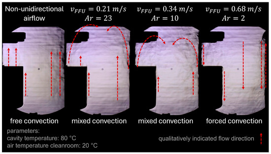
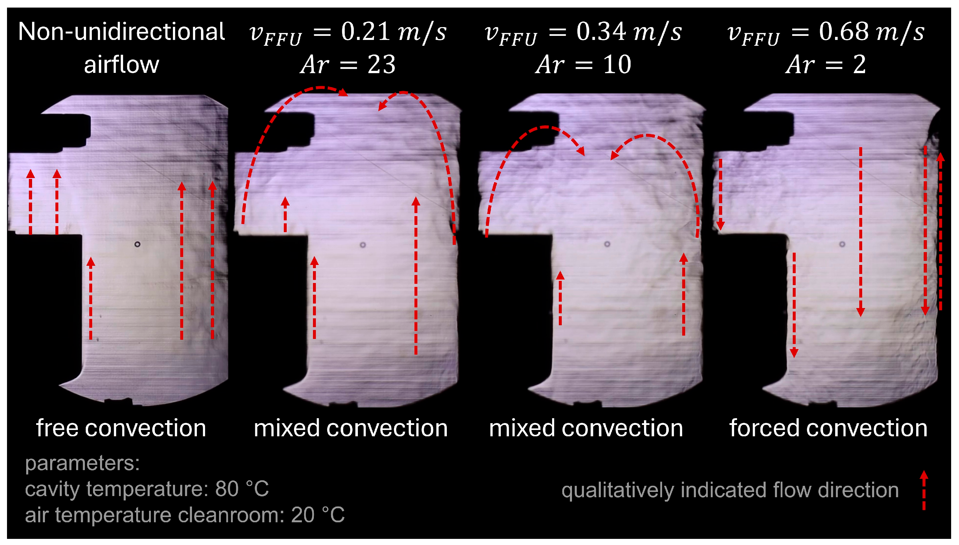
Figure 11 shows the flow visualization with schlieren photography at a mold set temperature (i.e., cavity temperature) of 80 °C. A video of the visualization showing the airflow regime in real time (duration 20 s) is attached in the Supplementary Material of this article. Without the use of an isolated region around the mold in a non-unidirectional airflow regime, the calculation of the Archimedes number is not possible. The airflow regime without FFU results in a free natural convection. Buoyancy plumes form on the front surfaces of the mold and rise freely. With the use of a FFU, a unidirectional downward airflow (opposed to free convection) is introduced. The interaction between free and forced convection becomes visible. For the lowest analyzed FFU velocity of , buoyancy plumes dominate the flow field. The Schlieren images show that the thermal plume is only partially deflected by the downward airflow and rises even on the horizontal surface of the cavity. In this regime, the plume penetrates the incoming FFU airflow and creates large recirculation structures above the mold. At an intermediate airflow velocity of , buoyancy and forced convection are of comparable magnitude. The Schlieren images indicate a transitional regime in which the rising thermal plume is significantly bent by the downward airflow, leading to complex recirculating flow structures in the mold region. At higher airflow velocities of , forced convection clearly dominates the flow field. The convective flow only establishes within the boundary layer. The downward airflow suppresses buoyancy plumes to rise above the mold height and transports the heated air downward along the mold surfaces. In this regime, the thermal plume no longer penetrates the unidirectional airflow, and the flow follows the imposed unidirectional direction.
Figure 11.
Schlieren photography of the mold cavity at a mold set temperature of 80 °C.
These observations illustrate how the relative strength of buoyancy and forced convection governs the airflow structure near the injection mold. The transition between buoyancy-dominated and forced-flow-dominated flow regimes is also reflected in the Archimedes number, which compares buoyancy and inertial forces in the flow. However, as shown in the literature, no critical Archimedes numbers could be derived merely by visual analysis of the flow. The transition between these regimes is particularly relevant for particle transport, as buoyancy-dominated flow structures can transport particles toward the mold cavity despite the downward cleanroom airflow.
3.3. Particle Contamination Dependent on Archimedes Number
As shown in the previous chapter, the Archimedes number can describe the flow regime of an isolated injection mold. While regulations like the EU-GMP [9] require a unidirectional airflow within critical areas assessed with failure mode and effects analysis, the effect of the flow regime on the risk of particle contamination needs to be analyzed. A link between the Archimedes number and the particle count within the isolated mold region is therefore analyzed.
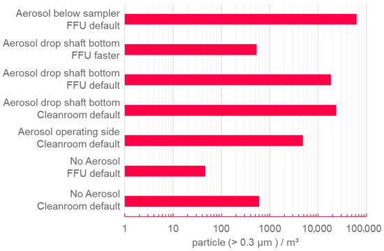
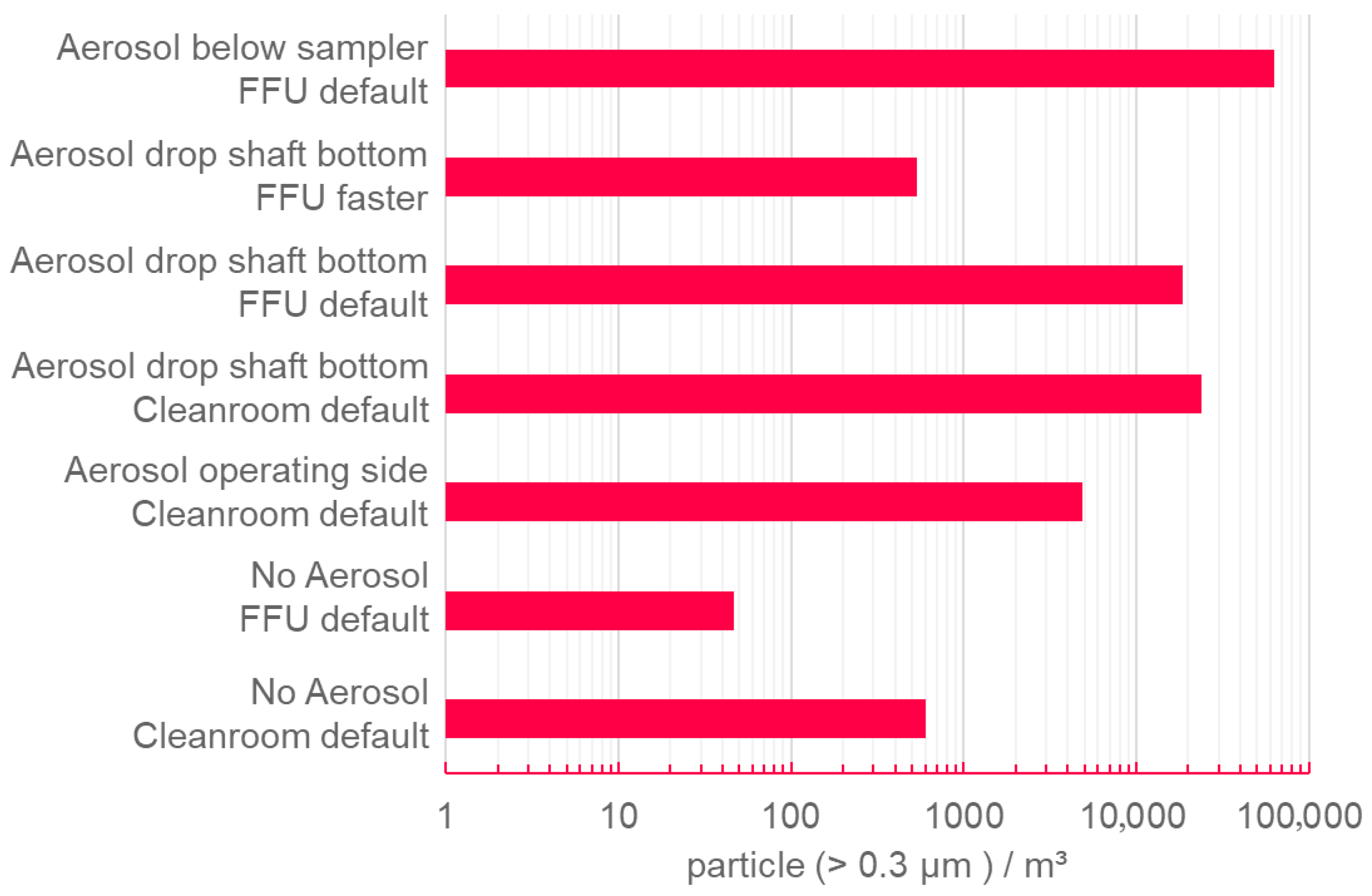
In preliminary tests, different positions of the aerosol injector and the resulting particles within the mold area were analyzed (Figure 12). The results show that particles injected outside the mold area (i.e., on the operating side of the machine) are transported into the mold area. This indicates that particles emitted within the cleanroom (e.g., personnel interacting with the injection molding machines user interface) can migrate into the mold area when not using an isolator with FFU around the mold. Emitting the particles inside the injection molding machines drop shaft further increased the number of particles. With the use of a FFU (), the particle count could be decreased, though cross contamination still occurred. The number of particles was further reduced by increasing the FFU’s volume flow. However, the particle concentration without an aerosol could not be reached. Therefore, preliminary tests highlight the danger of particles reaching the mold area and underline the state of the art for the justification of an isolated mold region, even when the injection molding production cell is placed in a cleanroom.
Figure 12.
Results of a preliminary test to determine the aerosol concentration within the mold area, depending on the location of the aerosol injection.
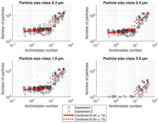
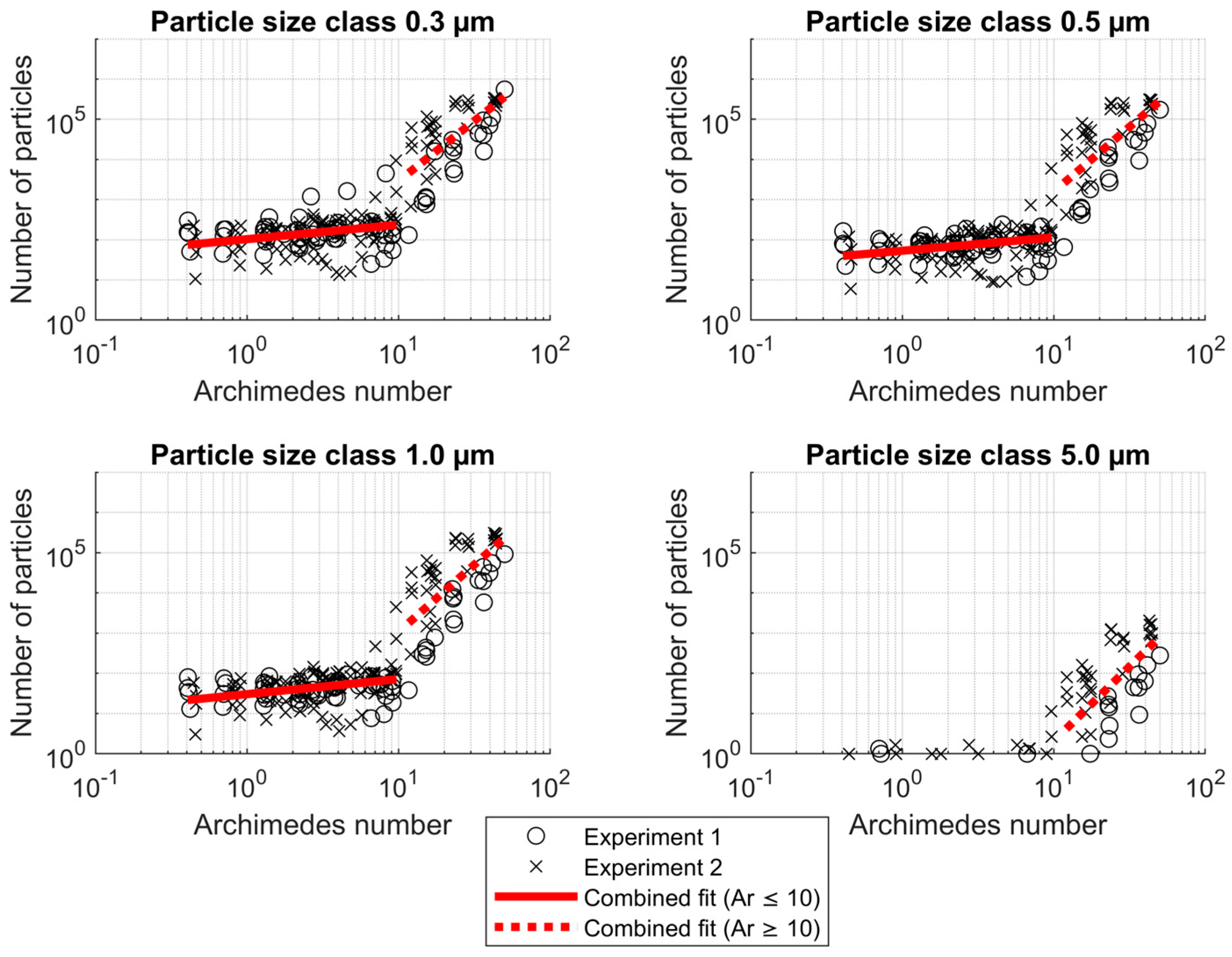
Further experiments were conducted to analyze the effect of different flow regimes within the mold area (described by the introduced Archimedes number) on the contamination risk (described by the amount of aerosol particles within the mold area). The experiments were conducted twice to ensure the reproducibility of the results. Figure 13 shows the particle load within the mold area for particle size classes of 0.3 µm, 0.5 µm, 1 µm and 5 µm. A clear trend is visible in both experiments: for Archimedes numbers less than 10, the particle count is low and nearly constant with scattering. The low particle count resembles the cleanroom background during experiments. Due to the injected aerosol and the presence of persons and measurement equipment in the room, the cleanroom background particle count was higher than in the standard operational state. For Archimedes numbers greater than ten, the particle count increases. The transitional flow regime can be observed over all particle size classes. Due to the small number of introduced aerosol particles of size ≥ 0.5 µm, the number of data points for the 5 µm particle size class is lower than for the smaller particle sizes. A slight difference between the two experiments suggests another dependent factor that was not included in the Archimedes number calculation, such as the exact position and orientation of the aerosol injection and the particle counter. The maximum values reached are approximately 10% of the particles injected by the aerosol. The flow regimes for different Archimedes numbers were also observed in the flow visualization in the previous chapter. Low Archimedes numbers with dominant forced convection have a low particle count, whereas high Archimedes numbers with dominant free convection have high particle counts. A transitional flow regime is consistently observed around an Archimedes number of across all particle size classes and in both experimental repetitions (compare Figure 13). In this region, the particle concentration begins to increase systematically, marking the onset of buoyancy-dominated transport into the mold area. The increase in particle concentration with an increasing Archimedes number suggests a continuous, potentially exponential relationship, rather than a discrete transition with a clearly defined mathematical turning point. Consequently, a unique critical value cannot be derived purely from curve fitting. Instead, defining the critical Archimedes number as the point at which a sustained increase in particle concentration occurs across all measured particle sizes, a threshold of approximately can be identified for the investigated mold geometry. This behavior is consistent with the gradual shift from forced- to buoyancy-dominated convection, rather than an abrupt regime change. The identified transition is supported not only by the particle measurements but also by the flow visualization results presented in the previous chapter, which show a shift from forced-convection-dominated to buoyancy-influenced flow structures in the same range. Despite minor deviations between the two experimental runs, the transition occurs within a narrow Archimedes number range. Higher particle counts shift to lower Archimedes numbers in the second experiment. Though a shift in flow regime and particle count is observed similar to the first experiment, a slightly different critical Archimedes number for both experiments can be observed. This underlines the sensitivity of the experiment to exact particle counter probe placing and orientation, as described in the results of the pretests. Additionally, this highlights that the observed critical value is a mere orientation without general validity. Nonetheless, above this threshold, particle concentrations increase significantly for all particle sizes, highlighting the relevance of buoyancy effects for contamination risk. While the exact threshold may vary with mold geometry, injection molding machine and FFU, the existence of a distinct transition between forced and buoyancy-dominated regimes is expected to remain. Due to the mentioned deviations in experiment repetition, the stated critical Archimedes number must be seen as a reference value for this specific setup, rather than a universally applicable threshold.
Figure 13.
Particle count within the mold area in dependency of the Archimedes number for the particle size classes 0.3 µm, 0.5 µm, 1 µm and 5 µm.
4. Conclusions
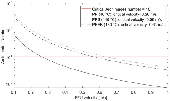
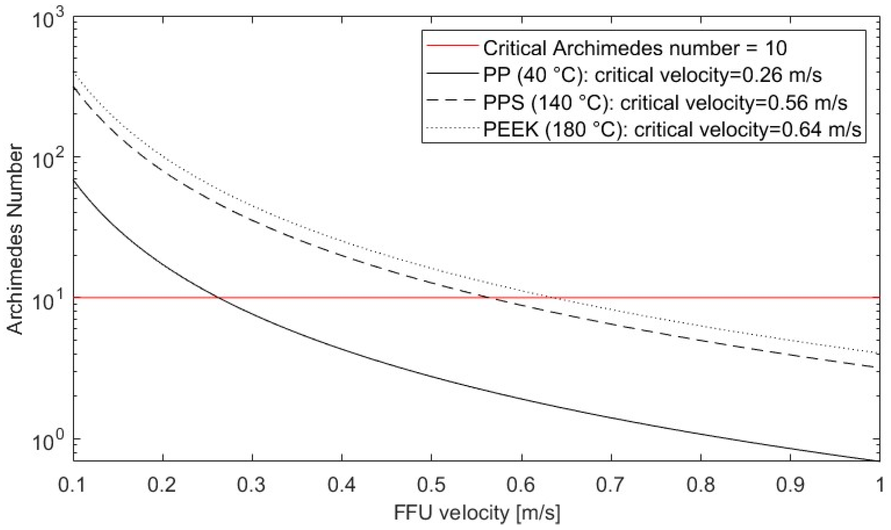
The present work introduces a simple procedure with only four measurement points to quantify the heat load of injection molding production cells. The measurements show that the heat load is significantly impacted by peripheral devices, and it increases with the mold set temperature. For the isolated injection molding machine (excluding the peripheral devices), the heat load is not significantly affected by the process and remains nearly constant. For the analyzed injection molding machines, the hydraulic machine has a lower heat load for comparable processes than the fully electrical machine. Furthermore, heat released by injection molds can significantly disturb the unidirectional airflow in cleanroom environments, generating buoyancy-driven plumes in the mold region. Cross contamination of particles is possible even when using a FFU and isolating the injection mold from the surrounding cleanroom airflow. The particle concentration in the mold area depends on several factors, which can be correlated with the Archimedes number. The experimental data indicate the existence of a critical Archimedes number above which a minimum FFU velocity is required to suppress convective effects. For the analyzed combination of injection molding machine, injection mold and FFU, this threshold was observed at . From this, design values for the necessary FFU volumetric flow rate can be derived for the analyzed injection mold. To date, cleanroom design guidelines prescribe fixed air velocities (e.g., 0.36–0.54 m/s for EU-GMP Grade A environments [9]) without explicitly accounting for thermally induced buoyancy effects caused by process equipment. The present work closes the gap caused by the lack of consideration of thermal effects by introducing an experimentally validated Archimedes number-based criterion that links process-specific heat loads and mold geometry to the required airflow conditions. Therefore, this approach provides a scientific justification (as required by the EU-GMP Contamination Control Strategy [9]) for selecting FFU airflow velocities outside the range of 0.36–0.54 m/s for injection molding applications inside cleanroom isolators. Additionally, the analysis method may support future cleanroom design optimization by linking case-specific heat loads and particle concentrations to Archimedes numbers. Using the analyzed injection mold as an example, Figure 14 relates the Archimedes number to FFU velocity for different process conditions, allowing a direct derivation of the minimum required airflow velocity to suppress convective effects. Depending on the mold set temperature, the minimum velocity ranges from 0.26 m/s up to 0.64 m/s, with both values outside the standard velocity range. Therefore, this approach allows the FFU to operate at lower velocities (i.e., optimal energy efficiency) and higher velocities (i.e., product safety). To the authors’ knowledge, no comparable experimentally derived critical Archimedes number for injection molding processes in cleanroom environments has been reported in the literature. The presented method therefore provides a first quantitative framework for assessing buoyancy-driven contamination risks in such systems.
Figure 14.
Archimedes number over FFU velocity of the analyzed injection mold for different polymers and corresponding mold set temperatures.
Currently, it can be concluded that the heat load generated by the injection molding machine and its peripherals depends on many factors and cannot be reliably predicted by simple calculations. However, it can be easily determined for a specific running process using the proposed method. The Archimedes number formulation presented here includes characteristic mold dimensions and heat flux as governing parameters. For molds with significantly different geometries, additional geometric factors may need to be considered. The value should therefore be interpreted as a first experimentally derived reference for injection molding applications, rather than a universal constant.
The almost similar energy consumption of the electrical and hydraulic machine is in direct contrast to general consensus in the literature [36,37,38,39]. Future research therefore should focus on the advancements of drive systems of injection molding machines and their effects on energy consumption and resulting heat loads. To make a clear recommendation for a specific injection molding machine type in cleanrooms (i.e., electrical, or hydraulic machine), additional measurements of different machines and processes are necessary, focusing on heat emitted into the surrounding. Additionally, the particle emission of the machine type as well as machine maintenance should be considered. There are still many factors to be investigated in future studies to provide recommendations and increase the energy efficiency and product safety of injection molding in cleanrooms. To determine a generally valid critical Archimedes number for injection molds in cleanrooms, additional data from different machines, molds, operating conditions and FFUs are required. To ensure high variation in mold geometries, additional data could be generated by computational fluid dynamics.
Overall, these findings highlight that thermal loads from injection molding machines must be considered not only in the design of cleanroom HVAC systems but also in contamination risk assessments for injection molding production cells. The presented Archimedes number-based approach provides a simple framework for assessing the risk of buoyancy-driven contamination in injection molding cleanrooms. From a practical perspective, buoyancy-driven disturbances can be mitigated by maintaining low Archimedes numbers: for example, by increasing the local airflow velocity where necessary. Therefore, it can contribute to scientifically justified air velocities other than 0.45 m/s ± 20% (EU-GMP Grade A environments) in contamination risk assessment, according to EU-GMP.
Supplementary Materials
The following supporting information can be downloaded at: https://www.mdpi.com/article/10.3390/atmos17050518/s1, Video S1: Schlieren visualization.
Author Contributions
Conceptualization, S.P., P.K. and S.R.; methodology, S.P.; validation, S.P.; formal analysis, S.P.; investigation, S.P.; data curation, S.P.; writing—original draft preparation, S.P.; writing—review and editing, S.P., P.K. and S.R.; visualization, S.P.; supervision, P.K. and S.R.; project administration, P.K. All authors have read and agreed to the published version of the manuscript.
Funding
This research was funded by Bundesministerium für Wirtschaft und Energie, grant number KK5209702KP1.
Institutional Review Board Statement
Not applicable.
Informed Consent Statement
Not applicable.
Data Availability Statement
The data presented in this study are available upon request from the corresponding author due to privacy restrictions.
Conflicts of Interest
The authors declare no conflicts of interest.
Abbreviations
The following abbreviations are used in this manuscript:
| DSC | Differential scanning calorimetry |
| FFU | Filter fan unit |
| HVAC | Heating, ventilation, and air conditioning |
| PP | Polypropylene |
| PPS GFR | Glass fiber reinforced Polyphenylene sulfide |
| TCU | Temperature control unit |
| Area | |
| Archimedes number | |
| Mold depth | |
| Electrical energy | |
| Gravitational constant | |
| Enthalpy | |
| Heat transfer coefficient | |
| Characteristic length | |
| Nusselt number | |
| Specific heating power | |
| Heat | |
| Heat flow | |
| Temperature | |
| Time | |
| Internal energy | |
| Work | |
| Velocity | |
| Thermal expansion coefficient of air | |
| Thermal conductivity | |
| Dimensionless factor |
Appendix A. Differential Scanning Calorimetry of the Processed Polymers
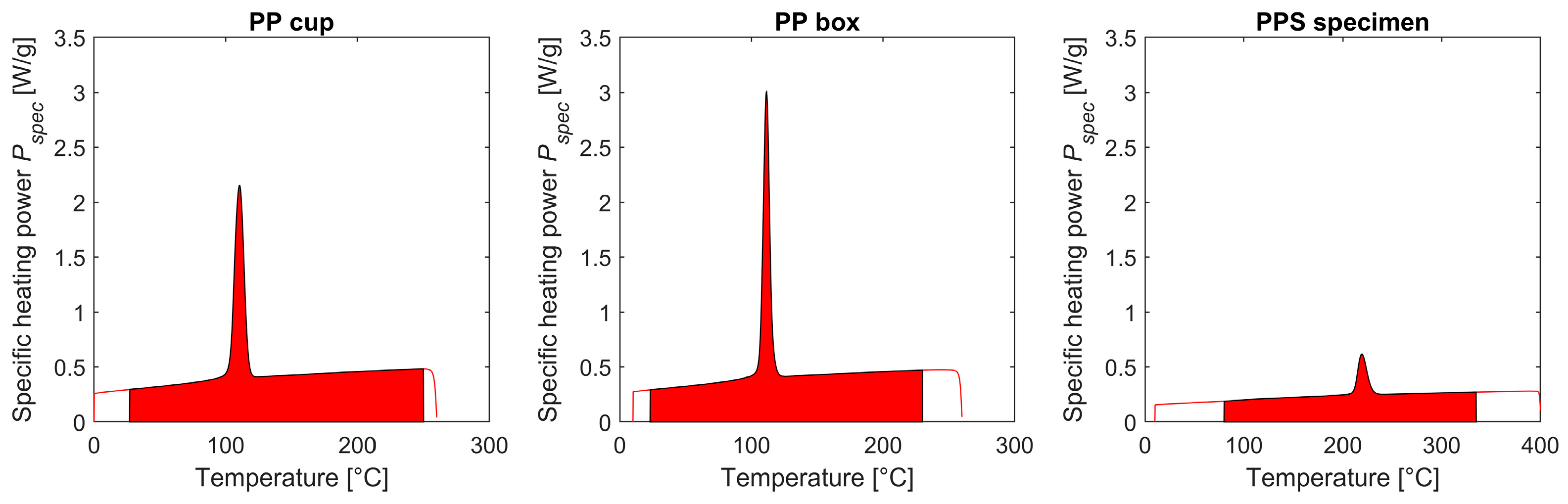
During a DSC measurement, the plastic is heated at a constant rate (10 K/min in this case) from a defined starting temperature to a target temperature. The specific power required for this process is recorded and plotted against the temperature. For the energy balance, the change in enthalpy refers to the temperature difference in the plastic from when it is fed into the injection molding machine (i.e., the plastification cylinder) to when it is injected into the mold. This equals the energy that is needed to heat and melt the plastic. This energy is transformed from the cylinder band heating and the screw movement (i.e., shear stress) into the plastic.
Since the temperature changes at a constant rate of 10 K/min throughout the measurement, the duration of the measurement and the temperature change are directly proportional to each other. Therefore, the time can be expressed as a function of the temperature . In other words, the temperature of the plastic can be assigned to specific points in time during the DSC measurement. Integrating the specific power measurement curve determines the enthalpy change in the plastic for two defined temperatures. This results in the following equation:
Here, is the temperature of the plastic granules at the feed point and is the temperature of the molten plastic during injection into the mold. The heat content of the injected plastic can be determined based on the mass of the processed plastic. Figure A1 shows the specific power for the processed polymers.
Figure A1.
Heating curve (red line) from a DSC measurement for different polymers with the specific enthalpy (red shadow) corresponding to each process.
References
- Bürkle, E.; Karlinger, P.; Wobbe, H. Reinraumtechnik in der Spritzgießverarbeitung; Carl Hanser Verlag GmbH & Co. KG: München, Germany, 2013. [Google Scholar]
- Permana, I.; Agharid, A.P.; Singh, N.; Wang, F. Full-scale evaluation of FFU configurations in an optical cleanroom injection molding for improving thermal performance and contaminant removal. Case Stud. Therm. Eng. 2024, 61, 105076. [Google Scholar] [CrossRef]
- Guo, Z.; Xie, J.; Yang, J.; Fu, J.; Zhao, P. Rapid mold temperature rising method for PEEK microcellular injection molding based on induction heating. J. Mater. Res. Technol. 2023, 26, 3285–3300. [Google Scholar] [CrossRef]
- Djunaedy, E.; van den Wymelenberg, K.; Acker, B.; Thimmana, H. Oversizing of HVAC system: Signatures and penalties. Energy Build. 2011, 43, 468–475. [Google Scholar] [CrossRef]
- DIN EN ISO 14644-1; Reinräume und Zugehörige Reinraumbereiche: Teil 1: Klassifizierung der Luftreinheit Anhand der Partikelkonzentration. DIN Deutsches Institut für Normung e. V.: Berlin, Germany, 2016.
- Amellal, K.; Tzoganakis, C.; Penlidis, A.; Rempel, G.L. Injection molding of medical plastics: A review. Adv. Polym. Technol. 1994, 13, 315–322. [Google Scholar] [CrossRef]
- Puntigam, S.; Karlinger, P. Einfluss der Abwärme des Spritzgusswerkzeugs auf die Produktion Unter Reinraumbedingungen; Technische Universität Chemnitz: Chemnitz, Germany, 2021. [Google Scholar]
- Bürkle, E.; Dittel, G. Produktionssicheres Spritzgießen im ISO5/GMP-A-Reinraum. Kunststoffe 2005, 95, 138–143. [Google Scholar]
- European Commission. The Rules Governing Medicinal Products in the European Union Volume 4 EU Guidelines for Good Manufacturing Practice for Medicinal Products for Human and Veterinary Use: Annex 1 Manufacture of Sterile Medicinal Products; C(2022) 5938 final; European Commission: Brussels, Belgium, 2022; Available online: https://health.ec.europa.eu/medicinal-products/eudralex/eudralex-volume-4_de (accessed on 21 January 2026).
- Schöngruber, H.; Lhota, C. Auf den Kopf gestellt: Neues Reinraumkonzept für Hochtemperaturanwendungen. Plastverarbeiter 2017, 14–18. Available online: https://a.storyblok.com/f/136567/x/50207737dd/2017-06-plastverarbeiter-auf-den-kopf-gestellt-de.pdf (accessed on 21 January 2026).
- Hofer, V. Zum Kontaminierten Raumvolumen von Partikel und Wärmequellen in Laminarer Verdrängungsströmung. Ph.D. Thesis, Technische Universität Berlin, Berlin, Germany, 2019. [Google Scholar]
- Stephan, P.; Kabelac, S.; Kind, M.; Mewes, D.; Schaber, K.; Wetzel, T. (Eds.) VDI-Wärmeatlas: Fachlicher Träger VDI-Gesellschaft Verfahrenstechnik und Chemieingenieurwesen, 12th ed.; Springer: Berlin/Heidelberg, Germany, 2019. [Google Scholar]
- Regenscheit, O.B. Strömungsvorgänge in Reinräumen und Rämen mit Reinfeldern. Chem. Ing. Tech. 1969, 41, 1050–1056. [Google Scholar] [CrossRef]
- Quarini, G.L.; Chang, Y.C.; Tierney, M.J.; Poulter, R. Characteristics and ‘Figures of Merit’ for the Value of the Ventilation in Clean Rooms. Chem. Eng. Res. Des. 1997, 75, 672–676. [Google Scholar] [CrossRef]
- Ding, L.C.; Yau, Y.H. A study on the arrangement of air inlets in a Class 7 clean room. Build. Serv. Eng. Res. Technol. 2015, 36, 357–367. [Google Scholar] [CrossRef]
- Yang, C.; Yang, X.; Zhao, B. The ventilation needed to control thermal plume and particle dispersion from manikins in a unidirectional ventilated protective isolation room. Build. Simul. 2015, 8, 551–565. [Google Scholar] [CrossRef]
- Schliesser, J.; Staudt-Fischbach, P. Minienvironments and thermal effects. In 10th Annual IEEE/SEMI. Advanced Semiconductor Manufacturing Conference and Workshop. ASMC 99 Proceedings (Cat. No.99CH36295); IEEE: Piscataway, NJ, USA, 1999; pp. 432–439. [Google Scholar]
- Li, X.; Liu, F.; Xie, J.; Zhang, C.; Gao, R.; Lyu, C.; Zhao, P. Research on metallic contamination control of PFA injection molded fittings. J. Appl. Polym. Sci. 2023, 140, e53940. [Google Scholar] [CrossRef]
- Weiß, P. Energieeffizienz und Abwärmenutzung in der Kunststoffverarbeitung. Ph.D. Thesis, Universität Duisburg-Essen, Duisburg-Essen, Germany, 2016. [Google Scholar]
- Eben, J.; Eigenbrod, H.; Karlinger, P.; Krallmann, K.; Kruppa, S.; Neher, J.; Peters, G.; Schiffers, R.; Würtele, M. Zustandsabhägige Prozessführung für die Energieeffiziente und Ressourcenschonenede Produktion von Kunststoffformteilen (ZuPrEff). Abschlussbericht 2012. [Google Scholar] [CrossRef]
- Liu, J. Erhöhung der Reproduzierbarkeit des Spritzgießprozesses Durch Verbesserte Plastifizierkonzepte. Ph.D. Thesis, Technische Universität München, München, Germany, 2009. [Google Scholar]
- Vormoor, N. Entwicklung, Durchführung und Bewertung Einer Methodik der Energieeffizienzmessung für eine Vollhydraulische Spritzgießmaschine in der Kunststoffindustrie. Ph.D. Thesis, Technische Universität Clausthal, Clausthal, Germany, 2017. [Google Scholar]
- Pamminger, R.; Wimmer, W.; Winkler, R.E. Energiedienstleistung zur Steigerung der Energieeffizienz von Spritzgießmaschinen im Kunststoffbereich; Bundesministerium für Verkehr, Innovation und Technologie: Wien, Austria, 2009. [Google Scholar]
- Pamminger, R.; Wimmer, W.; Winkler, R. Entwicklung von Kriterien zur Kommunikation der Energieeffizienz von Kunststoff Verarbeitenden Maschinen; Bundesministerium für Verkehr, Innovation und Technologie: Wien, Austria, 2010. [Google Scholar]
- Kaiser, W.; Schlachter, W. Energie in der Kunststofftechnik: Grundlagen und Anwendungen für Ingenieure; Carl Hanser Verlag München: München, Germany, 2019. [Google Scholar]
- Zhao, C.; Gao, F. Melt temperature profile prediction for thermoplastic injection molding. Polym. Eng. Sci. 1999, 39, 1787–1801. [Google Scholar] [CrossRef]
- Jeon, J.; Rhee, B.; Gim, J. Melt Temperature Estimation by Machine Learning Model Based on Energy Flow in Injection Molding. Polymers 2022, 14, 5548. [Google Scholar] [CrossRef]
- Puntigam, S.; Karlinger, P. Spritzgusswerkzeuge im Reinraum: Eine Analyse des Kamineffekts in der Kunststoffverarbeitung. Clean. Process. 2023, 2, 110–116. [Google Scholar]
- Sparrow, E.M.; Eichhorn, R.; Gregg, J.L. Combined Forced and Free Convection in a Boundary Layer Flow. Phys. Fluids 1959, 2, 319. [Google Scholar] [CrossRef]
- Wagner, W. Wärmeübertragung: Grundlagen, 7th ed.; überarb. u. erw. Aufl.; Vogel: Würzburg, Germany, 2011. [Google Scholar]
- Baehr, H.D.; Stephan, K. Wärme- und Stoffübertragung; Springer: Berlin/Heidelberg, Germany, 2019. [Google Scholar]
- Karwa, R. Heat and Mass Transfer, 2nd ed.; Springer: Singapore, 2020. [Google Scholar]
- Motegi, K.; Sibamoto, Y.; Hibiki, T.; Tsukamoto, N.; Kaneko, J. Opposing Mixed Convection Heat Transfer for Turbulent Single-Phase Flows. Int. J. Energy Res. 2024, 2024, 6029412. [Google Scholar] [CrossRef]
- Zhang, J.; Liu, J.; Lu, W. Study on Laminar Natural Convection Heat Transfer from a Hemisphere with Uniform Heat Flux Surface. J. Therm. Sci. 2019, 28, 232–245. [Google Scholar] [CrossRef]
- Settles, G.S. Colour-coding schlieren techniques for the optical study of heat and fluid flow. Int. J. Heat Fluid Flow 1985, 6, 3–15. [Google Scholar] [CrossRef]
- Thiriez, A. An Environmental Analysis of Injection Molding. Master’s Thesis, Massachusetts Institute of Technology, Cambridge, MA, USA, 2006. [Google Scholar]
- Nguyen, D.T.; Yu, E.; Barry, C.; Chen, W.-T. Energy consumption variability in life cycle assessments of injection molding processes: A critical review and future outlooks. J. Clean. Prod. 2024, 452, 142229. [Google Scholar] [CrossRef]
- Ribeiro, I.; Peças, P.; Henriques, E. Modelling the energy consumption in the injection moulding process. Int. J. Sustain. Manuf. 2015, 3, 289–309. [Google Scholar] [CrossRef]
- Elduque, A.; Elduque, D.; Clavería, I.; Javierre, C. Influence of material and injection molding machine’s selection on the electricity consumption and environmental impact of the injection molding process: An experimental approach. Int. J. Precis. Eng. Manuf. Green Technol. 2018, 5, 13–28. [Google Scholar] [CrossRef]
- Dr. Boy GmbH & Co. KG. Focus on Energy Efficiency: Servo-Hydraulics vs. Fully Electric Injection Moulding Machines. Available online: https://www.dr-boy.de/images/downloads-en/Mic/Focus_on_energy_efficiency__servo-hydraulics_vs__fully_electric_injection_molding_machines.pdf (accessed on 27 April 2026).

Disclaimer/Publisher’s Note: The statements, opinions and data contained in all publications are solely those of the individual author(s) and contributor(s) and not of MDPI and/or the editor(s). MDPI and/or the editor(s) disclaim responsibility for any injury to people or property resulting from any ideas, methods, instructions or products referred to in the content. |
© 2026 by the authors. Licensee MDPI, Basel, Switzerland. This article is an open access article distributed under the terms and conditions of the Creative Commons Attribution (CC BY) license.