


Abstract
Future volcanic eruptions are largely omitted from CMIP6 simulations, thereby increasing the uncertainty in 21st-century climate projections. We performed an 80-year (2020–2100) 25-member stochastic ensemble simulation with the climate model SOCOL-MPIOM, driven by the SSP3-7.0 forcing scenario, and introduced five stochastically distributed tropical eruptions—three strong, one moderate, and one weak—for each ensemble member (hereafter, SV run). We analyse volcanic influence by comparing the SV run results against a single volcanic-free baseline simulation under the same anthropogenic forcing scenario. Five eruptions over the 80-year simulation period leave the trends of the major climate indicators statistically indistinguishable from those of the volcanic-free baseline at the global and annual mean scales. However, on local and seasonal scales, volcanic activity can substantially alter the results of the volcanic-free simulation. For example, over Northern Europe, volcanic eruptions produce winter temperature warming of up to 1.0 K (about 30% of the warming in the reference run) and an annual precipitation deficit of 36 mm yr−1. This emphasises the need to include volcanic eruptions for more accurate projections of future climate. Probabilistic analysis of the SV ensemble shows that the annual maximum daily temperature (TXx) exceeds +0.5 K over 16% of global land with more-likely-than-not probability, a perturbation absent in standard CMIP6 results. Since our scenario composition targets the upper bound of plausible 21st-century volcanic activity, these exceedance areas represent near-maximum rather than most-probable estimates.
1. Introduction
Explosive volcanic eruptions inject sulphur dioxide (SO2) into the stratosphere, where it oxidises to form a sulphate aerosol layer. The aerosol particles enhance planetary albedo, suppress surface shortwave radiation, and absorb both incoming solar and outgoing terrestrial longwave radiation—warming the lower stratosphere while cooling the troposphere and surface [1,2]. These perturbations to the global energy budget trigger dynamical, chemical, and cryospheric responses that persist for months to years after a major eruption.
The observational and proxy record provides well-documented evidence across several events. The 1991 eruption of Mount Pinatubo—the largest stratospheric sulphur injection of the instrumental era—produced surface and tropospheric cooling of approximately 0.5 K within two years, accompanied by reduced global precipitation and a measurable ozone column perturbation through heterogeneous chemistry on aerosol surfaces [3,4,5,6]. The El Chichón (1982) and Tambora (1815) eruptions had analogous signatures in instrumental and proxy records [7,8].
Beyond the direct radiative effect, aerosol-induced heating of the tropical lower stratosphere steepens the equator-to-pole temperature gradient. It strengthens the polar vortex, favouring a positive Arctic Oscillation phase in the first post-eruption winters, warming the northern landmasses, and driving anomalous westerly advection over northern Eurasia [9,10,11]. This teleconnection is not uniformly reproduced across models: simulations tend to overestimate the polar vortex response at moderate forcing amplitudes [12,13], though the Eurasian winter warming pattern emerges consistently across eruption magnitudes in CMIP5 ensembles [14].
Sulphate aerosols also perturb stratospheric ozone chemistry by accelerating heterogeneous chlorine activation via ClONO2 + HCl → Cl2 + HNO3, depleting tropical ozone and redistributing polar ozone [4,15]. Heterogeneous N2O5 hydrolysis depletes reactive nitrogen oxide concentrations and can increase ozone concentrations above the aerosol layer [16]. Simultaneously, aerosol-induced stratospheric heating from infrared absorption modifies the Brewer–Dobson circulation and the poleward transport of ozone-rich air. The net ozone response reflects the balance between chemical destruction and dynamical transport. This balance depends on background halogen loading, which declines steadily as ozone-depleting substances are phased out under the Montreal Protocol [17].
At high latitudes, albedo feedback amplifies the surface response to volcanic eruptions: aerosol-induced cooling expands sea ice and snow cover, raising surface albedo and further suppressing temperatures [1,18,19]. Arctic sea-ice sensitivity to volcanic forcing is particularly relevant given the rapid contraction of the cryosphere under anthropogenic warming and the role of diminishing sea-ice cover in Arctic amplification [20,21].
Yet the cumulative climatic effect of recurrent volcanism over the full 21st century remains poorly quantified. Studies of catastrophic single eruptions—e.g., Pinatubo-class events injecting >10 Tg SO2—have dominated the literature, while the superposition of multiple eruptions each injecting 1–5 Tg SO2 over decadal to centennial timescales has received comparatively less attention, despite such events dominating the historical frequency distribution [22]. Most CMIP6 integrations either omit future volcanic forcing or prescribe a constant background aerosol climatology, underestimating the uncertainty range of possible climate trajectories [23,24,25]. No century-scale stochastic volcanic ensemble has yet coupled interactive ozone chemistry to prescribed volcanic aerosol forcing across the full atmosphere [2,26]. Volcanic forcing superimposed on a warming background state may also produce nonlinear responses in threshold-sensitive systems such as the Arctic sea-ice margin and the monsoon belt [27,28], and climate change is itself expected to modify the stratospheric lifetime and radiative efficiency of volcanic aerosol [29], providing another source of nonlinearity that single-eruption experiments cannot capture.
To address this gap, we conducted an 80-year, 25-member stochastic ensemble simulation using a chemistry-climate model driven by the SSP3-7.0 emission scenario for the period 2020–2100. Previous stochastic volcanic studies have either employed reduced-complexity frameworks [25] or lacked interactive stratospheric chemistry [26]. This study extends these approaches by providing the first characterisation of the centennial volcanic climate signal within a fully coupled chemistry-climate model that simultaneously resolves interactive stratospheric ozone chemistry, prescribed aerosol radiative and heterogeneous-chemistry forcing, ocean-sea-ice coupling, and regional climate extremes. Each ensemble member incorporates five eruptions with independently sampled magnitudes and timings. The volcanic signal is isolated by subtracting the volcanic-free baseline from the ensemble mean. It is examined in the context of background ozone and temperature trends, vertical and meridional structures, regional surface climate, cryospheric feedbacks, climate extremes as defined by the Expert Team on Climate Change Detection and Indices (ETCCDIs), and the probabilistic exceedance of warming thresholds.
2. Materials and Methods
2.1. Model Description
SOCOL-MPIOM couples the atmospheric chemistry-climate model SOCOL to the ocean-sea-ice model MPIOM through the OASIS3 interface, exchanging fields daily. The atmospheric component builds on the ECHAM5.4 general circulation model [30], extended with the MEZON interactive stratospheric chemistry scheme, which treats 41 chemical species in 140 gas-phase, photolytic, and heterogeneous reactions—including the full halogen and nitrogen oxide catalytic cycles governing ozone chemistry [31]. The model runs at spectral resolution T31 (≈3.75° × 3.75°) with 39 vertical levels from the surface to 0.01 hPa (~80 km). The oceanic component MPIOM uses a bipolar grid at approximately 3° horizontal resolution with 40 vertical levels. Stratospheric sulphate aerosol size distributions (SAD) and optical properties are prescribed to account for radiative forcing and heterogeneous ozone chemistry.
Model performance has been assessed against observational and reanalysis data in several validation studies [32,33,34]. The SOCOL-MPIOM reproduces large-scale temperature and circulation patterns over the historical period, though it tends to overestimate global surface warming during the industrial era [33]. The model captures the global-scale ozone and temperature response to major volcanic eruptions, including Pinatubo (1991), but, as with other chemistry-climate models, it overestimates lower-stratospheric warming following large events [35,36]. The atmospheric component (ECHAM5 coupled with MEZON) has been validated against ERA5 and MERRA-2 reanalyses, showing good agreement in temperature and stratospheric ozone trends over 1980–2020 [37].
2.2. Experimental Design
The baseline is a single transient run over 2020–2100 under the SSP3-7.0 forcing scenario, with no volcanic forcing beyond a constant background stratospheric aerosol optical depth. Greenhouse gas (CO2, CH4, N2O) concentrations follow the SSP3-7.0 data. Solar irradiance follows the standard reconstructions consistent with CMIP6 protocols [38]. SSP3-7.0, with a radiative forcing of +7.0 W m−2 by 2100, was selected to maximise the signal-to-noise ratio for detecting the volcanic perturbation against internal variability.
The volcanic ensemble (SV) comprises 25 independent members, each realising five tropical eruptions over 2020–2100. All members share the baseline boundary conditions and initial conditions, with volcanic aerosol forcing as the sole source of inter-member difference. For each eruption, time-dependent forcing is prescribed as three-dimensional fields of aerosol optical depth, specific surface area, and scattering and absorption parameters (extinction, single-scattering albedo, asymmetry factor) in NetCDF format at T31L39 resolution. Aerosol properties and distributions are derived from Arfeuille et al. [39]. Since aerosol optical properties are prescribed from a historical library rather than interactively simulated, potential feedbacks between the evolving background climate state and aerosol microphysics or lifetime are not captured in this framework—a limitation discussed further in Section 4.9.
2.3. Construction of Stochastic Volcanic Scenarios
Scenario construction draws on the eruption record spanning the 10th to 20th centuries compiled by Toohey et al. [40], which documents 55 events classified by maximum stratospheric aerosol optical depth (AOD) in the eruption year: strong (AOD > 0.10), moderate (0.05 < AOD ≤ 0.10), and weak (AOD ≤ 0.05). Century-by-century statistics are given in Table 1; the long-term mean is five eruptions per century, approximately two strong, one moderate, and two weak.
Table 1.
Century-by-century statistics of volcanic eruptions from the 10th to 20th centuries based on Toohey et al. [40]. Classification by maximum stratospheric aerosol optical depth (AOD): strong (AOD > 0.10), moderate (0.05 < AOD ≤ 0.10), weak (AOD ≤ 0.05).
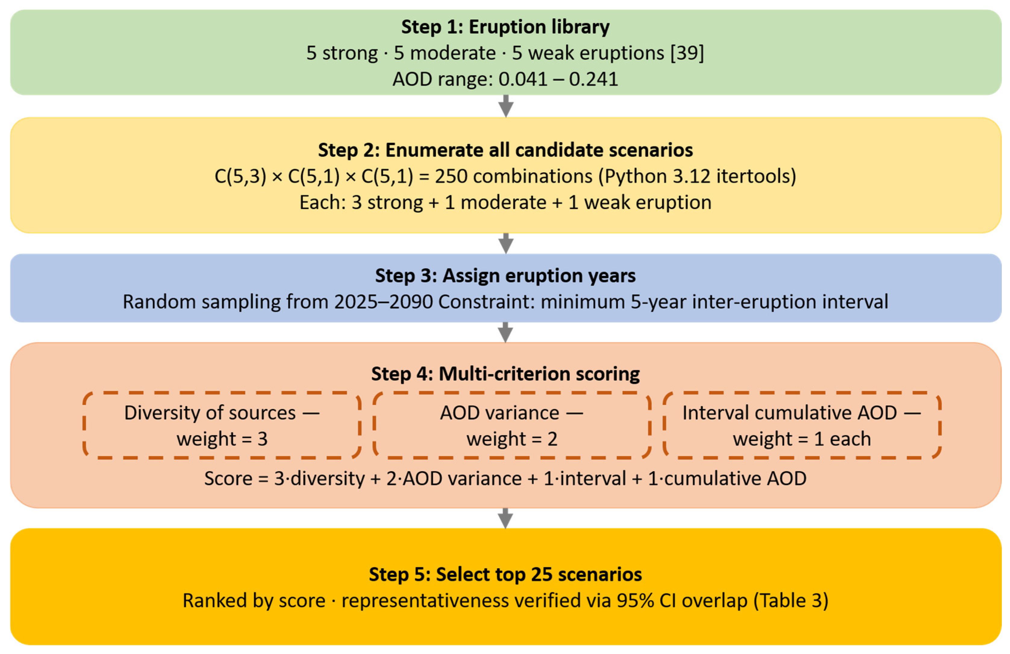
Aerosol forcing fields are taken from [41], covering 1600–2020, and include detailed stratospheric aerosol characterisation for 15 eruptions (Table 2). To target the upper bound of historical variability and maximise signal detectability, each 21st-century scenario contains three strong, one moderate, and one weak eruption. All within-category combinations were enumerated exhaustively (Python 3.12 standard library module itertools), producing 250 candidate scenarios. Eruption years are drawn randomly over 2020–2090, subject to a minimum five-year inter-eruption interval to prevent aerosol superposition outside the forcing library’s calibration range. The full selection procedure is summarised in Figure A2 (Appendix B). All injections are assigned tropical latitudes, consistent with the eruption class that produces a globally distributed stratospheric aerosol layer.
Table 2.
Volcanic eruptions from [39] used to construct future volcanic scenarios, classified by maximum stratospheric AOD in the eruption year.
A subset of 25 scenarios was selected from the 250 candidates using a multi-criterion scoring function designed to preserve the statistical distribution of the full pool while reducing computational cost by a factor of ten. The scoring function weighted four criteria: diversity of volcanic sources (weight 3), variance of total aerosol loading (weight 2), correspondence of the inter-eruption interval distribution to the pool means (weight 1), and correspondence of cumulative AOD to the pool mean (weight 1). Representativeness was verified by comparing 95% confidence intervals for mean peak AOD, mean inter-eruption interval, and cumulative AOD between the full pool and the selected subset (Table 3); overlapping intervals in all three parameters confirm that the 25 scenarios constitute an unbiased sample of possible 21st-century volcanic histories.
Table 3.
Comparison of key statistical parameters between the full sample of 250 candidate scenarios and the 25 selected scenarios. Values are given as mean ± 95% confidence interval. Overlapping intervals confirm that the selected subset is statistically representative of the full sample.
2.4. Definition of the Volcanic Signal
For each ensemble member i, the volcanic signal is defined as the difference from the baseline:
Spatial and temporal analyses use the ensemble-mean signal:
Statistical significance is assessed by a one-sample t-test on the 25 member-wise anomalies ΔXi, testing whether their mean differs from zero. The baseline enters as a fixed estimate of the volcanic-free forced trajectory; this approach follows established practice in large-ensemble studies, where a single control run serves this role [42]. Throughout this study, reported p-values and significance masks should be interpreted as diagnostic estimates of the volcanic signal relative to a fixed baseline trajectory, rather than as formal detection thresholds against a fully sampled no-volcano counterfactual.
2.5. Statistical Methods
At each grid point, the significance of the volcanic signal is evaluated by a two-tailed Student’s t-test at the 5% level (p < 0.05), comparing the 25 SV values against the baseline over 2090–2100. Ensemble spread is summarised by the 5th–95th inter-member percentile range. Long-term linear trends over 2020–2100 are estimated by ordinary least squares for both the SV ensemble mean and the baseline, and significance is assessed using the Mann–Kendall test. Pearson correlation coefficients between domain-averaged annual time series are computed over the full 2020–2100 period and flagged at three levels: p < 0.05 (*), p < 0.01 (**), and p < 0.001 (***).
Probabilistic exceedance maps are constructed from the 25-member distribution: for each grid point and threshold τ, the exceedance probability is the fraction of members for which ΔX > τ. The 50% contour (more likely than not) and 75% contour (high confidence, following IPCC AR6 robustness criteria [43]) are shown in all exceedance maps.
2.6. Climate Extreme Indices
Changes in climate extremes are quantified using a subset of ETCCDIs [44]: the annual maximum of daily maximum temperature (TXx), the annual minimum of daily minimum temperature (TNn), the diurnal temperature range (DTR), the fraction of warm days (TX90p), frost days (FD), summer days (SU), and total annual precipitation (PRCPTOT). All indices are computed from daily model output for each ensemble member and differenced against the baseline over the 2090–2100 versus 2020–2030 period.
Regional averages are computed over eight domains: the Arctic (>66° N), Northern Europe (50–70° N, 10–40° E), Central Asia (35–55° N, 60–90° E), East Asia (25–45° N, 100–140° E), the Tropics (30° S–30° N), North America (25–60° N, 130–60° W), the Southern Hemisphere (<30° S), and the Antarctic (<60° S).
2.7. EOF Analysis of the Northern Hemisphere Temperature Mode
We apply empirical orthogonal function (EOF) analysis to monthly near-surface temperature (T2m) and atmospheric surface pressure (APS) poleward of 20° N, separately for boreal winter (DJF) and summer (JJA). December is assigned to the following calendar year for DJF compositing. EOF patterns are derived exclusively from the baseline simulation, such that the volcanic signal does not influence the covariance structure.
Seasonal anomalies are linearly detrended and weighted by √cos φ before decomposition. The leading EOF (EOF1) is extracted by singular value decomposition and normalised to unit variance. For T2m, the sign convention follows the standard AO definition in temperature space: negative loadings over the Arctic correspond to the AO+ pattern, in which a positive principal component reflects a cold Arctic and warm mid-latitudes.
The volcanic signal is projected onto EOF1 by regressing the area-weighted ensemble-mean anomaly field (SV minus baseline) onto the EOF1 pattern at each year over 2020–2100. The resulting projection coefficient time series (ΔPC1) tracks the extent to which volcanic forcing excites or suppresses the leading mode. Because the EOF pattern is normalised to unit variance and the anomaly field retains its original units (K for T2m, hPa for APS), ΔPC1 carries the units of the original variable (K and hPa, respectively), representing the amplitude of the volcanic anomaly projected onto the leading mode. For T2m, a negative ΔPC1 indicates a warm-Arctic, cool mid-latitude departure; for APS, a positive ΔPC1 indicates a low-pressure anomaly over the Arctic consistent with AO+. Statistical significance is assessed by a one-sample t-test on the 25 member-wise ΔPC1 values against zero (p < 0.05).
3. Results
3.1. Background Trends: Volcanic Versus Non-Volcanic Simulations
Century-scale trends in both experiments provide the climatic context for interpreting the volcanic perturbation (Figure 1). Over 2020–2100, the SV ensemble mean and the baseline track each other closely across all four variables; recurrent stochastic eruptions leave no detectable imprint on the long-term trajectory of the climate system under SSP3-7.0.
Figure 1.
Long-term trends in stratospheric ozone, tropospheric ozone, stratospheric temperature, and near-surface temperature over 2020–2100 in the SV ensemble and the volcanic-free baseline simulation. (a) Stratospheric O3 mixing ratio (50–10 hPa, ppmv). (b) Tropospheric O3 mixing ratio (1000–850 hPa, ppbv). (c) Stratospheric temperature (50–10 hPa, K). (d) Near-surface temperature (1000–850 hPa, K). In each panel, the dark blue line shows the 25-member SV ensemble mean with ±1σ spread (light blue shading); the dark red line shows the volcanic-free baseline (SSP3-7.0). Dashed lines indicate ordinary least-squares linear trends for each experiment, with trend values and significance levels annotated in the lower right of each panel. Orange vertical shading marks years in which the SV ensemble mean and the baseline differ significantly (p < 0.05, two-tailed Student’s t-test). All four trends are significant at p < 0.001 (***).
Stratospheric ozone (50–10 hPa) increases in both experiments—+0.009 ppmv dec−1 in SV and +0.006 ppmv dec−1 in the baseline (both p < 0.001; Figure 1a)—consistent with ongoing ozone layer recovery under the Montreal Protocol. The large interannual variability driven by QBO dynamics limits the explained variance in both cases (R2 = 0.40 and 0.20); a 5-year running mean is applied in Figure 1a to aid visual interpretation of the long-term signal.
Tropospheric ozone (1000–850 hPa) declines at −1.440 and −1.459 ppbv dec−1 in SV and baseline, respectively (both p < 0.001, R2 = 0.96; Figure 1b). Stratospheric temperature decreases at −0.420 and −0.411 K dec−1 (Figure 1c), and surface temperature increases at +0.338 and +0.341 K dec−1 (Figure 1d). Across all four variables, the absolute differences between the two experiments are negligibly small and fall within the range attributable to internal model variability rather than a systematic volcanic forcing effect. Five eruptions over the 80-year simulation period—comprising three strong, one moderate, and one weak event, and thus representing the upper bound of plausible 21st-century volcanic activity—leave no detectable imprint on the centennial trajectory of any global-mean variable under SSP3-7.0, confirming that the volcanic signal at the global scale does not manifest as a long-term trend shift.
3.2. Temporal Evolution and Vertical Structure of the Volcanic Signal
The volcanic signal over 2020–2100 shows pronounced interannual variability superimposed on a weakly positive stratospheric offset and a weakly negative near-surface offset (Figure 2, left panels). Stratospheric temperature anomalies average +0.181 K with a peak of +0.626 K in 2060 (Figure 2a), consistent with aerosol-induced radiative heating of the lower stratosphere. The discrete warm pulses of 0.3–0.6 K, separated by near-zero intervals, reflect stochastic eruption timing across members. Near-surface temperature is negative on average (mean −0.051 K; Figure 2c), with ensemble spread substantially exceeding the mean in any given year. Stratospheric ozone increases secularly through the century (mean +0.010 ppmv; Figure 2e), with consistently positive anomalies emerging after 2060 as background halogen loading declines and volcanic perturbations to ozone chemistry shift toward net production. However, the signal-to-noise ratio for the stratospheric ozone anomaly is moderate (S/N = 0.59; Appendix A), reflecting large QBO-driven interannual variability in the baseline; significance statements for this variable should therefore be interpreted with appropriate caution.
Figure 2.
Temporal evolution and vertical structure of the volcanic signal (SV ensemble mean minus baseline) over 2020–2100 for three key variables. Left panels: time series of globally averaged volcanic anomalies smoothed with a 5-year running mean (dark blue line); light blue shading denotes ±1σ ensemble spread; orange shading indicates years with significant anomaly (p < 0.05, one-sample t-test). Mean and peak anomaly values are annotated in the upper left of each panel. The horizontal line marks zero anomaly. (a) Stratospheric temperature anomaly (50–10 hPa, K). (c) Near-surface temperature anomaly (850–1000 hPa, K). (e) Stratospheric O3 mixing ratio anomaly (50–10 hPa, ppmv). Right panels: vertical profiles of the volcanic anomaly from the surface to ~80 km (0.01 hPa) for three sub-periods (2020–2040, blue solid; 2040–2070, purple dashed; 2070–2100, red dotted) and the full-period mean (black bold line); ±1σ shading applies to the full-period mean; filled circles mark levels with significant anomaly (p < 0.05). The horizontal dashed line indicates the climatological tropopause (~12 km). (b) Temperature anomaly profiles (K). (d) Global-mean O3 mixing ratio anomaly profiles (ppmv). (f) O3 mixing ratio anomaly profiles by latitude zone: Tropics (30° S–30° N, red), NH mid-latitudes (30–60° N, light blue), NH polar region (60–90° N, dark blue). Sub-period means (dashed lines) reflect the evolving background climate; the average number of eruptions per sub-period across the 25 members is 1.4 (2020–2040), 1.8 (2040–2070), and 1.8 (2070–2100).
The vertical temperature profile is dominated by a warming maximum at approximately 16–20 km (Figure 2b). The global-mean signal peaks near +0.4 K at 18 km; tropical latitudes experience the largest warming (+0.7–1.0 K), where sulphate aerosol concentration and longwave absorption are greatest. Above 25 km, the anomaly decreases rapidly and becomes statistically indistinguishable from zero in the upper stratosphere and mesosphere. In the troposphere, significant cooling of −0.3 to −0.5 K is present at 10–6 km, reflecting reduced shortwave transmission. The vertical profile shape is reproduced consistently across all three sub-periods (2020–2040, 2040–2070, 2070–2100), indicating that the thermal response structure does not depend on the background climate state.
The ozone vertical profile shows a two-tier structure (Figure 2d,f). In the tropical lower stratosphere (16–20 km), the signal is negative, reaching −0.02 ppmv at peak levels—the zone of maximum aerosol surface area density where heterogeneous chlorine activation depletes ozone most efficiently. In the polar middle stratosphere (30–45 km), a positive anomaly develops, reaching +0.05 ppmv in the NH polar region by the end of the century. The tropical deficit deepens slightly from 2020–2040 to 2070–2100, while the polar surplus grows as declining background halogens reduce chemical ozone loss sensitivity and enhanced poleward transport under the volcanically perturbed Brewer–Dobson circulation progressively enriches polar air.
The meridional extent and vertical boundaries of these two regimes are resolved in the zonal-mean latitude-pressure section for 2090–2100 (Figure 3).
Figure 3.
Zonal-mean latitude-pressure section of the volcanic ozone signal (ΔO3 = SV ensemble mean minus baseline) averaged over 2090–2100. Grey stippling marks grid points where the anomaly is not statistically significant (p > 0.05, two-tailed Student’s t-test on 25 member-wise anomalies). The dashed line at 100 hPa marks the approximate extratropical tropopause. The red bracket indicates the region of mid-stratospheric polar enrichment (20–50 hPa); the black bracket marks the lowermost stratosphere (LMS, 100–200 hPa). Tropical depletion (up to −40 ppbv) is confined to the 70–200 hPa layer, where aerosol surface area density is highest. Poleward of 30° N and above 50 hPa, the signal reverses, reaching +40 ppbv in the NH polar middle stratosphere—the region where ozone-rich air accumulates under the strengthened Brewer–Dobson circulation. No systematic positive anomaly appears in the LMS (100–200 hPa) at any latitude, ruling out enhanced stratosphere-troposphere exchange as the mechanism behind the attenuated tropospheric ozone trend discussed in Section 4.1.
3.3. Spatial Distribution and Seasonal Dependence
The total ozone column anomaly (ΔTOZ) for 2090–2100 relative to 2020–2030 shows a meridionally banded pattern: tropical latitudes lose 2–5 DU while high latitudes of both hemispheres gain 3–8 DU (Figure 4a; 65% of grid points show anomalies detectable relative to the baseline). This structure is the column-integrated expression of the two-tier vertical ozone profile documented in Section 3.2. Surface temperature anomalies (ΔT2max, ΔT2min) are predominantly positive across the Northern Hemisphere extratropics, reaching +0.5 to +1.5 K over the Arctic and northern Eurasia, with near-zero or weakly negative values over tropical and subtropical continents (Figure 4b,c; 68% of grid points show anomalies detectable relative to the baseline).
Figure 4.
Spatial distribution of the volcanic signal (SV ensemble mean minus baseline) for the period 2090–2100 relative to 2020–2030. (a) Total ozone column anomaly ΔTOZ (Dobson units). (b) Annual maximum daily maximum temperature anomaly ΔT2max (K). (c) Annual minimum daily minimum temperature anomaly ΔT2min (K). (Grey shading indicates grid points where the anomaly is not statistically significant (p > 0.05, two-tailed Student’s t-test). (d) Diurnal temperature range DTR (K) The percentage of grid points with a significant anomaly is shown in the lower right of each panel.
The seasonal decomposition reveals that two physically distinct mechanisms govern the regional response (Figure 5). In boreal winter (DJF), the dominant feature in the temperature field is a warming of +1.0 to +2.0 K over Northern Europe and the broader Eurasian sector, detectable relative to the baseline over 72% of the domain (Figure 5a). This pattern is spatially consistent with the stratospheric teleconnection pathway: aerosol-induced heating of the tropical lower stratosphere steepens the equator-to-pole temperature gradient, intensifies the polar vortex, and drives anomalous westerly advection of warm Atlantic air over northern Eurasia [9,10,14]. DJF precipitation over Northern Europe shows a corresponding weak positive anomaly of +2.0 mm season−1 (Figure 5c), physically consistent with enhanced moisture transport under the same westerly circulation anomaly. A direct attribution to a specific AO phase requires geopotential height diagnostics, which are not available in the present dataset; the EOF-based characterisation of the Northern Hemisphere temperature mode is presented in Section 3.7.
Figure 5.
Seasonal dependence of the volcanic signal in surface temperature and precipitation for 2090–2100 relative to 2020–2030. (a,b) Annual maximum daily maximum temperature anomaly ΔT2max (K) for DJF and JJA. (c,d) Total seasonal precipitation anomaly ΔPRCPTOT (mm season−1) for DJF and JJA. Grey shading indicates grid points where the anomaly is not statistically significant (p > 0.05). Black rectangle in (a) and red rectangles in (c,d) delineate Northern Europe (50–70° N, 10–40° E); dashed lines in (b) indicate the tropical belt (30° S–30° N). The contrasting patterns between DJF and JJA reflect the transition from stratospheric teleconnection-driven warming in winter to direct aerosol radiative suppression of convection in summer.
In boreal summer (JJA), the stratospheric pathway is inactive, and the surface response is controlled by direct aerosol radiative forcing. Tropical and subtropical land surfaces cool by −0.5 to −1.0 K (Figure 5b) as volcanic aerosol attenuates incoming shortwave radiation at latitudes of peak summer insolation. Over Northern Europe, JJA precipitation decreases by −10.6 mm season−1 (Figure 5d), reflecting suppressed convective activity under reduced surface heating rather than any circulation-driven anomaly. The annual precipitation deficit of −36 mm yr−1 over Northern Europe therefore combines a dynamically driven DJF moistening and a radiatively driven JJA drying, the latter dominating the annual total. Globally, precipitation falls by −2.0 mm yr−1 (p < 0.001), concentrated over northern mid-latitude continental interiors and subtropical convergence zones.
3.4. Cryospheric Feedback Mechanism
The high-latitude surface response is governed by a cryospheric feedback chain, quantified through correlation analysis of the 25-member ensemble time series (Figure 6).
Figure 6.
Quantification of the cryospheric feedback chain linking volcanic aerosol forcing to Arctic surface response. Left column: time series of globally or Arctic-averaged volcanic signal anomalies (2020–2100, 5-year running mean, dark blue; ±1σ, light blue shading; yellow = significant years, p < 0.05). The horizontal line marks zero anomaly. Significance levels are denoted by asterisks: *** p < 0.001 (a) Surface shortwave radiation anomaly ΔSW (W m−2). (d) Arctic sea-ice area anomaly Δseaice (%). Centre column: spatial maps of the volcanic signal (2090–2100 vs. 2020–2030) in polar stereographic projection (60–90° N). (b) ΔSW surface (W m−2). (e) Δseaice (%). Right column: scatter plots of ensemble-mean annual anomalies over 2020–2100. (c) ΔSW surface vs. Δseaice Arctic (%); the Pearson correlation r = −0.50 (p < 0.001) is shown; the additional correlation between cloud cover anomaly (Δaclcov) and ΔSW surface (r = −0.63, p < 0.001) is annotated. (f) Global mean surface albedo anomaly ΔAlbedo vs. Arctic minimum temperature anomaly ΔT2min (K); r = −0.89 (p < 0.001). Red lines show ordinary least-squares regression fits in all scatter plots.
Volcanic reduction in surface shortwave radiation (Δsrads) is negative throughout most of the period (Figure 6a), with an Arctic spatial distribution mirroring the sea-ice response (Figure 6b). The correlation between Δsrads and Arctic sea-ice area is r = −0.50 (p < 0.001; Figure 6c); an additional correlation between cloud cover anomaly and surface shortwave (r = −0.63, p < 0.001) indicates that both direct aerosol attenuation and aerosol-induced cloudiness contribute to reduced surface insolation. Arctic sea-ice extent increases by +0.44% on average (p < 0.001) relative to the baseline (Figure 6d,e), with the largest anomalies in the Barents and Kara Seas.
The feedback closes through the surface albedo response. Arctic surface albedo anomalies correlate with Arctic minimum temperature (ΔT2min) at r = −0.89 (p < 0.001), with a regression slope of −0.016 albedo units per K (Figure 6f): volcanic surface cooling drives proportional sea-ice and snow expansion, which amplifies the initial cooling through elevated reflectivity. No analogous feedback operates in the tropics or subtropics, where surface albedo is insensitive to the snow-ice phase transition, confining this mechanism to high latitudes.
3.5. Volcanic Signal in Climate Extremes
The ETCCDI anomalies show a strongly heterogeneous regional structure (Figure 7). Global-mean values are small—ΔTXx = +0.03 K, ΔTNn = −0.02 K, ΔDTR = −0.01 K, ΔPRCPTOT = −0.0 mm yr−1—because opposing regional signals largely cancel at the global scale.
Figure 7.
Regional summary of the volcanic signal across nine geographic domains and ten ETCCDIs. Cell colours are normalised per column to the range [−1, +1] to highlight the relative spatial pattern; cell values show the absolute volcanic signal in the units of each index. Significance levels are denoted by asterisks: * p < 0.05, ** p < 0.01, *** p < 0.001. Regions: Global, Arctic (>66° N), Northern Europe (50–70° N, 10–40° E), Central Asia (35–55° N, 60–90° E), East Asia (25–45° N, 100–140° E), North America (25–60° N, 130–60° W), Tropics (30° S–30° N), Southern Hemisphere (<30° S), Antarctic (<60° S). Indices: DTR (K), TXx (K), TNn (K), FD (%), SU (%), ID (%), TR (%), TX90p (%), TN10p (%), PRCPTOT (mm yr−1).
Northern Europe shows the most consistent response across the domain: all 10 indices show anomalies significant relative to the fixed baseline, including TXx +0.74 K (p < 0.001), TNn +0.37 K (p < 0.05), DTR +0.10 K (p < 0.001), SU +12% (p < 0.001), FD −7.3% (p < 0.001), ID −13% (p < 0.001), TR +26% (p < 0.001), TX90p +3.15% (p < 0.001), TN10p −1.79% (p < 0.001), and PRCPTOT −36 mm yr−1 (p < 0.001)—the largest regional precipitation anomaly in the analysis. The warming-and-drying pattern, with increased warm days and reduced frost and ice days, is physically consistent with the DJF stratospheric teleconnection signal described in Section 3.3.
The Arctic shows the largest nocturnal warming: TNn reaches +0.66 K (p < 0.001), amplified through the cryospheric feedbacks documented in Section 3.4. Daytime warming is also significant but weaker (TXx +0.32 K, p < 0.001). Ice days decrease by −3.0% (p < 0.001) and frost days by −3.5% (p < 0.001), while cold-night frequency (TN10p) falls by −0.88% (p < 0.001). Total precipitation increases by +19 mm yr−1 (p < 0.001), partly reflecting enhanced moisture convergence into the warming Arctic.
Central Asia and East Asia show divergent responses. In Central Asia, the dominant signal is nocturnal cooling (TNn −0.73 K, p < 0.001) with increased frost and ice days (FD +11%, ID +12%; both p < 0.001) and a rise in cold-night frequency (TN10p +1.36%, p < 0.001), pointing to amplified winter continentality. Daytime extremes also warm significantly (TXx +0.27 K, p < 0.001), thereby widening the diurnal cycle. East Asia, by contrast, shows daytime warming (TXx +0.34 K, p < 0.001) with more summer days (+12%, p < 0.001) and warm days (TX90p +1.66%, p < 0.001), while nocturnal temperatures are not significantly affected—a pattern physically distinct from the night-time continental cooling in Central Asia.
In the tropics, direct aerosol suppression of surface insolation produces the only region of consistent daytime cooling: TXx −0.18 K (p < 0.001) and TX90p −1.27% (p < 0.001). Tropical precipitation increases by +3.1 mm yr−1 (p < 0.001), consistent with partial recovery of convective activity as surface cooling reduces the direct radiative deficit. North America shows no statistically significant response in any index, a result examined in Section 4.6.
3.6. Probabilistic Assessment
The 25-member ensemble allows the volcanic signal to be expressed as exceedance probabilities, following the IPCC AR6 robustness framework in which 50% defines “more likely than not” and 75% defines “high confidence” [45]. These thresholds provide a physically interpretable measure of how consistently the volcanic forcing exceeds a given magnitude across ensemble members, independent of the ensemble-mean signal strength. With n = 25 ensemble members, the binomial 95% confidence interval for an observed exceedance fraction of 50% spans approximately [30%, 70%], and for 75% spans [52%, 88%]. These intervals are wide relative to the thresholds, reflecting the moderate ensemble size; however, the spatial coherence of the signal—with exceedance probabilities exceeding 64% concentrated systematically over northern Eurasia and the Arctic rather than distributed randomly—indicates that the diagnosed patterns reflect forced responses rather than sampling artefacts. A bootstrap resampling analysis (10,000 iterations) confirms the binomial confidence intervals reported above, yielding identical 95% CIs of [29%, 71%] for the 50% exceedance fraction and [58%, 92%] for the 75% fraction—the agreement reflects the fact that the binomial approximation is exact for this ensemble size. A Monte Carlo field significance test (1000 sign-permutation iterations, preserving the spatial autocorrelation structure of the ensemble) confirms that the diagnosed spatial pattern cannot be attributed to random sampling noise: the observed fraction of significant NH grid points (76.1%) far exceeds the 99th percentile of the null distribution (44.3%), yielding p < 0.001.
For TXx warming above +0.5 K, the 50% threshold is exceeded over approximately 16% of global land (Figure 8a), concentrated in northern Eurasia, the Arctic, and parts of East Africa. The 75% contour, indicating high-confidence warming, covers 7% of the land area and is largely confined to northern Scandinavia and central Siberia. These regions spatially coincide with the areas of strongest ensemble-mean TXx anomaly identified in Section 3.5, confirming that the Northern Europe and Arctic signals are not artefacts of a few outlier members but reflect a consistent forced response across the ensemble. Raising the threshold to +1.0 K (Figure 8b) reduces the area exceeding 50% probability to 4%, with the 75% contour covering less than 1%. At +1.5 K (Figure 8c), neither criterion is met anywhere. The rapid probability dropoff between +0.5 K and +1.5 K reflects the moderate forcing regime: individual eruptions produce TXx anomalies well below the Pinatubo-class response, and the regional signal accumulates through the superposition of multiple events rather than through a single dominant perturbation. Since our scenarios target the upper end of plausible 21st-century eruption frequencies, the diagnosed exceedance areas should be read as near-maximum rather than most-probable estimates; a historically representative eruption composition would yield lower probabilities.
Figure 8.
Probabilistic assessment of the volcanic signal derived from the 25-member SV ensemble. Maps show the fraction of ensemble members for which the end-of-century volcanic signal (2090–2100 vs. 2020–2030) exceeds a given threshold. (a) Probability of TXx warming exceeding +0.5 K. (b) Probability of TXx warming exceeding +1.0 K. (c) Probability of TXx warming exceeding +1.5 K. (d) Probability of Arctic sea-ice area increase exceeding +1%, shown in polar stereographic projection (40–90° N). In all panels, thin black contours delineate the 50% probability level (“more likely than not”), and thick black contours delineate the 75% probability level (high confidence threshold following IPCC AR6 robustness criteria [43]). The percentage of the domain area exceeding the 50% and 75% thresholds is annotated in the lower right of each panel. The colour scale runs from 0% (white) to 100% (dark red).
For Arctic sea-ice, the probability of a +1% increase in area coverage exceeds 50% over parts of the Barents, Kara, and Laptev Seas (Figure 8d), with the 75% contour covering approximately 1% of the Arctic domain. The spatial pattern of high-confidence sea-ice response aligns with the regions of strongest shortwave reduction and cryospheric feedback identified in Section 3.4. Unlike the TXx signal, which shows a sharp probability dropoff with threshold, the sea-ice response is among the most spatially coherent features of the volcanic signal across ensemble members—a consequence of the tight physical coupling between aerosol-induced shortwave reduction and sea-ice area quantified by the albedo-temperature correlation (r = −0.89; Section 3.4). This robustness has direct relevance to near-term Arctic predictability: future volcanic eruptions may systematically interrupt the secular sea-ice decline projected under SSP3-7.0, a phenomenon absent from standard CMIP6 integrations.
3.7. EOF Analysis of the Northern Hemisphere Temperature and Pressure Modes
To characterise how the volcanic signal projects onto the leading modes of Northern Hemisphere atmospheric variability, EOF analysis was applied separately to near-surface temperature (T2m) and atmospheric surface pressure (APS) poleward of 20° N, for DJF and JJA (Section 2.7; Figure 9).
Figure 9.
EOF analysis of Northern Hemisphere near-surface temperature (T2m) and atmospheric surface pressure (APS), and their volcanic signal projections. (a) Spatial pattern of the leading EOF (EOF1) of DJF T2m poleward of 20° N, derived from the baseline simulation (19.5% of interannual variance explained); loadings are weighted by √cos φ. (b) Spatial pattern of EOF1 of DJF APS poleward of 20° N, derived from the baseline simulation (32.4% of interannual variance explained); the annular structure corresponds to the Arctic Oscillation in pressure space (AO+ phase: low pressure over the Arctic, high pressure over mid-latitudes). (c) Time series of the volcanic signal projection onto T2m-EOF1 (ΔPC1_T2m = SV ensemble mean minus baseline, K) for DJF (blue) and JJA (red), 2020–2100; ±1σ ensemble spread is shown by shading; years of significant anomaly (p < 0.05, one-sample t-test) are shaded in orange. (d) As (c) but for the projection onto APS-EOF1 (ΔPC1_APS, hPa). The robust DJF ΔPC1_T2m, paired with insignificant ΔPC1_APS, shows that the Arctic-warming mode in the temperature field does not depend on AO excitation in the pressure field.
The leading EOF of T2m (Figure 9a) explains 19.5% of the interannual variance and exhibits a regional dipole structure, with negative loadings over the North Atlantic–European sector and positive loadings over northern Russia and the Arctic. The projection of the volcanic anomaly onto this mode (ΔPC1_T2m; Figure 9c) is negative on average in DJF (mean = −3.69 K), indicating that the volcanic ensemble systematically shifts the near-surface temperature field toward a warm-Arctic, relatively cool North Atlantic–European pattern in boreal winter, consistent with the cryospheric amplification documented in Section 3.4. In JJA, ΔPC1_T2m is positive (mean = +2.19 K), reflecting the direct radiative cooling of mid-latitude land surfaces by tropical aerosol, which projects onto the opposite EOF1 pole in summer.
The leading EOF of APS (Figure 9b) explains 32.4% of the interannual variance—substantially more than its temperature counterpart—and exhibits the canonical annular structure of the Arctic Oscillation in pressure space: a deep negative loading centred over the pole and a positive loading over the Northern Hemisphere mid-latitudes, corresponding to the AO+ phase.
The projection of the volcanic anomaly onto APS-EOF1 (ΔPC1_APS; Figure 9d) oscillates around zero in both DJF and JJA, with no statistically significant mean offset in either season (p > 0.05). The ensemble spread substantially exceeds the ensemble mean throughout 2020–2100, and no systematic trend in ΔPC1_APS emerges across sub-periods.
The contrasting results for the two modes—robust non-zero ΔPC1_T2m versus statistically insignificant ΔPC1_APS—indicate that the dominant volcanic influence on the Northern Hemisphere winter temperature field does not arise from a coherent annular circulation shift. The warm-Arctic thermodynamic signal captured by ΔPC1_T2m is driven by sea-ice and snow-albedo feedbacks (Section 3.4). At the same time, the stratospheric teleconnection pathway, which would be expected to project positively onto APS-EOF1 through an intensified polar vortex, does not produce a detectable pressure-mode response at the moderate forcing amplitudes studied here. This decomposition into thermodynamic and dynamical components is discussed further in Section 4.8.
4. Discussion
4.1. Volcanic Forcing and the Centennial Warming Trend
The near-identical surface warming trends in the volcanic ensemble and the baseline (+0.338 vs. +0.334 K dec−1) confirm that five eruptions over the 80-year simulation period leave no detectable imprint on the centennial temperature trajectory under SSP3-7.0. Chim et al. [25] reached the same conclusion using the FaIR reduced-complexity climate model across three emission scenarios (SSP1-1.9, SSP2-4.5, SSP5-8.5): stochastic volcanic forcing shifts the ensemble-mean GMST by less than 0.1 °C relative to a constant-forcing baseline. The agreement between these two results is notable given the difference in model complexity. FaIR is an impulse-response framework calibrated to CMIP6 ensemble statistics, without explicit representation of atmospheric dynamics, stratospheric chemistry, or ocean-sea-ice coupling. SOCOL-MPIOM resolves all three. The fact that both approaches yield indistinguishable long-term warming trends suggests that the insensitivity of the centennial mean to moderate volcanic forcing is a robust physical result rather than an artefact of model simplification. At the same time, the regional signals documented in Section 3.3, Section 3.4 and Section 3.5 and the stratospheric ozone response described below fall entirely outside the diagnostic scope of reduced-complexity frameworks and require the mechanistic resolution provided by a coupled chemistry-climate model.
The tropospheric ozone trends in the SV ensemble and the baseline are likewise indistinguishable (−1.440 vs. −1.430 ppbv dec−1; Figure 1b), with the small numerical difference falling within the range of internal model variability. This result is not self-evident: the mid-stratospheric polar enrichment documented in Figure 3—driven by enhanced poleward transport under the volcanically perturbed Brewer–Dobson circulation—could in principle supply additional ozone to the troposphere via downward stratosphere-troposphere exchange (STE), partially offsetting the anthropogenic decline. The zonal-mean section (Figure 3) rules this pathway out directly: the polar enrichment above 50 hPa does not propagate into the lowermost stratosphere (LMS, 100–200 hPa), which remains near zero at all latitudes. Since the LMS is the primary gateway for downward ozone flux into the troposphere, the vertical discontinuity between the mid-stratospheric enrichment and the tropopause region confirms that enhanced STE plays no role in the tropospheric ozone budget under the forcing regime studied here.
4.2. Vertical Structure and the Century-Scale Evolution of the Ozone Response
The two-tier ozone profile—tropical depletion at 100–50 hPa paired with polar enrichment at 5–20 hPa—is consistent in structure with observations following Pinatubo (1991), where mid-latitude column reductions of 2–7% were recorded [1,4]. The ensemble-mean tropical deficit of −0.02 ppmv is considerably smaller, as expected for eruptions injecting 1–5 Tg SO2 rather than the ~20 Tg of Pinatubo. The physically significant result is not the amplitude but the century-scale amplification of the polar surplus: as stratospheric chlorine concentrations fall under the Montreal Protocol, the ozone response to volcanic aerosol shifts from net heterogeneous destruction toward net dynamical transport, with polar enrichment becoming the dominant feature of the volcanic ozone profile by 2070–2100. This evolution—from a chemistry-dominated to a transport-dominated regime—cannot be captured in single-eruption experiments and represents a qualitative change in the character of volcanic ozone forcing over the 21st century. Given the moderate signal-to-noise ratio of the stratospheric ozone signal (S/N = 0.59; Appendix A), this conclusion should be interpreted as indicative rather than definitive, and would benefit from confirmation with a volcanic-free ensemble.
4.3. Stratospheric Teleconnection and the Winter Warming of Northern Europe
The DJF warming over Northern Europe—exceeding +1.0–2.0 K in the ensemble mean, with all 10 ETCCDIs showing anomalies significant relative to the fixed baseline— is the most spatially coherent regional signal in the dataset. Its structure is consistent with the stratospheric teleconnection pathway: aerosol-induced heating of the tropical lower stratosphere steepens the equator-to-pole temperature gradient, strengthens the polar vortex, and shifts the midlatitude westerlies poleward, increasing warm Atlantic air advection over northern Eurasia in boreal winter [9,10,11]. This DJF warming pattern, accompanied by cooling over continental Central Asia, is reproduced across a range of eruption magnitudes in CMIP5 simulations [14] and in observational composites following Pinatubo, El Chichón, and Agung [11].
Two caveats apply. First, CMIP5 analyses indicate that models overestimate the polar vortex response to moderate volcanic forcing [12,13], suggesting that the diagnosed warming magnitude is likely an upper bound. Second, and more fundamentally, the EOF-based decomposition of temperature and pressure modes (Section 3.7) shows that the volcanic signal does not project significantly onto the AO pressure mode, indicating that the warm-Arctic temperature pattern reflects thermodynamic cryospheric amplification rather than a coherent circulation shift. The fact that the Northern Europe warming nonetheless emerges robustly across 72% of the DJF domain in a 25-member ensemble suggests that the dynamical pathway contributes to the regional surface temperature signal even when its pressure-mode expression falls below the detection threshold—a distinction that underscores the value of analysing temperature and pressure EOFs jointly.
The concurrent nocturnal cooling over Central Asia (TNn −0.73 K, p < 0.001) represents the dynamical counterpart of the European warming: enhanced westerly advection warms maritime Northern Europe while amplifying continentality over Central Asian interiors under the same circulation anomaly, consistent with the observed temperature response to positive AO conditions [46].
4.4. Cryospheric Feedbacks and Arctic Amplification
The feedback chain quantified in Section 3.4—aerosol shortwave reduction driving sea-ice expansion, which amplifies the initial cooling through elevated surface albedo (r = −0.89, p < 0.001)—shares its essential structure with the mechanism invoked to explain the onset of the Little Ice Age. Repeated explosive eruptions between 1275 and 1300 AD triggered sea-ice expansion that persisted for centuries through ocean-sea-ice feedbacks long after aerosol dissipation [19]. The present results operate in a far weaker forcing regime, and the sea-ice increase of +0.44% is small relative to the projected secular loss under SSP3-7.0. Nevertheless, the response is robust across ensemble members (>50% probability over key Arctic marginal seas; Figure 8d) and is physically linked to the aerosol radiative perturbation rather than to internal oceanic variability.
The practical implication is that future volcanic eruptions may repeatedly and temporarily interrupt the secular Arctic sea-ice decline, introducing a source of interannual-to-decadal variability currently absent from standard CMIP6 projections. This is relevant both to near-term Arctic predictability and to the attribution of observed sea-ice anomalies in the post-eruption period.
4.5. Precipitation Response and the Hydrological Cycle
The globally averaged precipitation reduction of −2.0 mm yr−1 (p < 0.001) and the pronounced Northern Europe deficit of −36 mm yr−1 (p < 0.001) are consistent with the volcanic hydrological response in CMIP5 multi-model analyses: robust drying over northern mid-latitude continental interiors, with European precipitation modulated by the atmospheric circulation response to volcanic forcing [47]. The land-ocean contrast in the hydrological response—land precipitation suppressed more rapidly than oceanic precipitation—also agrees with the Tambora-forced response in MIROC-ES2L [48].
The annual Northern Europe deficit integrates two physically distinct seasonal contributions: a dynamically driven DJF moistening (+2.0 mm season−1) and a radiatively driven JJA drying (−10.6 mm season−1), the latter dominating the annual total. This seasonal decomposition is important for impacts assessment: a region experiencing net annual drying may simultaneously see wetter winters and drier summers, with opposing implications for agriculture, water resources, and wildfire risk.
The comparatively weak tropical PRCPTOT signal (+3.1 mm yr−1, p < 0.001), despite the tropics being the primary aerosol injection zone, reflects partial compensation: as convective activity diminishes under surface cooling, reductions in cloud cover partially offset the direct shortwave deficit. This partial compensation between reduced convective activity and cloud cover changes is resolved in SOCOL-MPIOM through the coupled cloud-radiation scheme.
4.6. North America: Absence of a Detectable Signal
No statistically significant volcanic signal emerges in any ETCCDI over North America, a result that warrants physical interpretation rather than dismissal. For a one-sample t-test with n = 25 members and an ensemble spread of σ = 0.19 K over the North American domain, the minimum detectable signal at 80% power and p < 0.05 is 0.11 K—confirming that the ensemble has adequate statistical power to detect signals of this magnitude. The near-zero ensemble-mean anomaly (ΔTXx = +0.08 K, p = 0.05) therefore reflects genuine cancellation of competing dynamical pathways rather than insufficient statistical power. North America lies at the intersection of the AO/NAO pattern, which would tend to produce DJF warming as in Europe, and the Pacific–North America (PNA) teleconnection associated with ENSO variability, which generates opposing anomalies across different parts of the continent [1,46]. The stochastic eruption timing randomises the ENSO state at eruption onset, and the resulting interference across 25 members averages to zero. Unlike Northern Europe, where the stratospheric teleconnection pathway consistently dominates, North American climate extremes are not robustly modified by the moderate volcanic forcing class studied here.
4.7. Moderate Versus Catastrophic Eruptions: What Stochastic Ensembles Add
Single large-eruption studies—Pinatubo, Tambora, El Chichón—have established the mechanistic framework for volcanic climate impacts, but catastrophic eruptions (>10 Tg SO2) represent a small fraction of the expected 21st-century eruption frequency. A Tambora-sized event carries a roughly 10% probability of occurrence within any 50-year window [49], implying that the century is statistically dominated by the moderate-to-large regime represented in this ensemble. The stochastic approach quantifies what single-eruption studies cannot: the probability distribution of regional climate responses given realistic uncertainty in eruption timing, magnitude, and sequence. The probabilistic exceedance analysis (Figure 7) establishes that TXx warming of +0.5 K is more likely than not over ~16% of global land. Meanwhile, the probability drops to near zero at +1.5 K—a constraint that complements rather than contradicts the larger signals found in catastrophic eruption experiments and that is directly applicable to near-term climate risk assessment.
4.8. EOF Analysis: Thermodynamic Versus Dynamical Pathways of the Northern Hemisphere Volcanic Response
The combined EOF analysis of T2m and APS (Section 3.7, Figure 8) resolves a structural ambiguity central to volcanic attribution studies: whether the post-eruption winter warming over Northern Europe and the Arctic arises primarily from the stratospheric teleconnection pathway—aerosol heating of the tropical lower stratosphere intensifying the polar vortex and driving surface AO+—or from the cryospheric amplification pathway through sea-ice and albedo feedbacks. The results yield a clear answer at the moderate forcing amplitudes studied here: ΔPC1_APS is statistically insignificant throughout 2020–2100, while ΔPC1_T2m is robustly negative in DJF, demonstrating that the thermodynamic rather than the dynamical pathway dominates the Northern Hemisphere volcanic winter signal in this ensemble.
This finding is physically coherent with the moderate eruption regime. The stratospheric teleconnection requires the aerosol-induced lower-stratospheric warming to be sufficiently sustained to shift the meridional temperature gradient, strengthen the polar vortex, and couple downward to the surface on the monthly timescales relevant to the AO. At injection magnitudes of 1–5 Tg SO2, the lower-stratospheric warming signal is present (Section 3.2, peak +0.7–1.0 K in the tropical lower stratosphere). However, it appears insufficient to systematically exceed the noise threshold for a coherent pressure-mode response across the 25 ensemble members. This is consistent with analyses of CMIP5 volcanic ensembles, which find that models overestimate the polar vortex response even for Pinatubo-class forcing [13], implying that the true response at moderate forcing should be correspondingly weaker and less detectable. Bittner et al. [13] demonstrate with a 100-member MPI-ESM ensemble that detecting a significant NH polar vortex strengthening after the Pinatubo eruption requires at least 15 ensemble members, and that the response to El Chichón—approximately one third the SO2 loading of Pinatubo—remains statistically indistinguishable from zero even with 100 members. The eruptions in the present ensemble fall within this sub-Pinatubo forcing regime, providing an independent expectation that no coherent pressure-mode response should emerge at the 25-member ensemble size used here.
Conversely, the cryospheric amplification mechanism operates independently of any circulation anomaly: aerosol shortwave reduction directly lowers Arctic surface temperatures, expands sea ice, and amplifies the initial cooling through increased surface albedo (r = −0.89 between Arctic albedo and minimum temperature anomalies; Section 3.4). This mechanism requires no specific phase of the AO and is therefore detectable in the temperature EOF even when the pressure EOF shows no systematic response.
The higher explained variance of APS-EOF1 (32.4%) compared with T2m-EOF1 (19.5%) reflects the greater spatial coherence of the AO pressure signal relative to regional temperature variability. The fact that the volcanic forcing fails to project significantly onto the more coherent and statistically dominant pressure mode further reinforces the conclusion that the thermodynamic pathway governs the Northern Hemisphere response at this forcing level. This partitioning has direct implications for detection and attribution. A detectable positive AO signal in future pressure reanalyses following volcanic events would indicate a forcing regime substantially stronger than the moderate eruptions characterised here. It would be physically distinguishable from the thermodynamic warm-Arctic signal already documented in the present ensemble.
The positive JJA ΔPC1_T2m (+2.19) and the corresponding absence of a JJA pressure signal jointly confirm that the summer volcanic response is entirely radiative: aerosol suppression of surface insolation cools mid-latitude land surfaces without generating any associated circulation anomaly in either season.
4.9. Limitations and Outlook
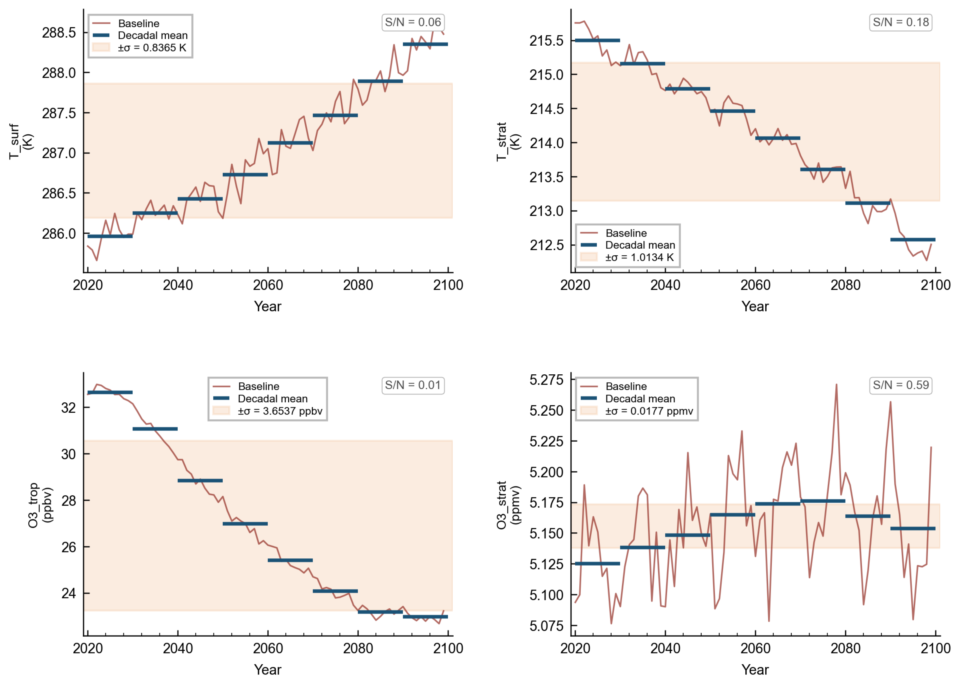
Several structural features of the experimental design warrant explicit discussion. The use of a single baseline simulation rather than a volcanic-free ensemble means that internal variability in the baseline introduces a common offset across all 25 member-wise anomalies ΔXᵢ, inflating the ensemble mean without affecting its variance; the one-sample t-test used here is therefore slightly anti-conservative. Signal-to-noise ratios estimated from decadal variability in the baseline confirm that this offset is negligible for near-surface and stratospheric temperature and for tropospheric ozone, but moderate for stratospheric ozone (S/N = 0.59; Figure A1), where QBO-driven interannual variability is large. Significance statements for stratospheric ozone are interpreted accordingly.
The scenario composition—three strong, one moderate, and one weak eruption per member, against a historical mean of approximately two strong events per century—deliberately targets the upper bound of plausible volcanic activity to maximise signal detectability. The diagnosed signal magnitudes should therefore be read as near-maximum rather than most-probable estimates. A complementary ensemble sampling the historically expected eruption composition would be needed to derive unbiased regional projections.
Three further limitations relate to model configuration. The absence of residual circulation diagnostics (v*, w*) precludes unambiguous attribution of polar ozone enrichment to enhanced Brewer–Dobson transport versus chemical mechanisms. The coarse horizontal resolution (T31, ≈3.75°) likely limits the fidelity of regional teleconnection patterns, particularly over orographically complex regions such as Central Asia, and may underestimate precipitation sensitivity to volcanic forcing [48]. All eruptions are assigned tropical injection latitudes; high-latitude events such as Laki (1783) produce distinct hemispheric asymmetries not represented here [1].
The QBO is prescribed from historical observations rather than simulated interactively, introducing an additional source of uncertainty since the QBO phase at eruption onset modulates stratospheric aerosol transport and the polar vortex response [50,51]. However, the practical significance of this limitation for the central conclusions of this study is constrained by the sub-Pinatubo forcing regime of the ensemble. Using a 100-member ensemble of MPI-ESM historical simulations, Bittner et al. [52] showed that at least 15 ensemble members are required to detect a statistically significant NH polar vortex strengthening after the Pinatubo eruption, and that the response to El Chichón—at approximately one-third the SO2 loading of Pinatubo—remains undetectable even with 100 members. Azoulay et al. [53] further demonstrated the existence of a forcing threshold between 2.5 and 5 Tg(S) below which the polar vortex shows no detectable response, using idealised 100-member ensembles. Since the individual eruptions in the present stochastic ensemble fall well below the Pinatubo SO2 loading, the AO pressure-mode response is already undetectable at the ensemble size used here regardless of QBO phase. A fixed QBO phase may, therefore, introduce uncertainty in individual member responses but is unlikely to affect the ensemble-mean conclusion of no significant AO excitation.
A further limitation concerns the prescribed nature of the volcanic aerosol forcing. Aerosol optical properties and surface area densities are taken from a historical forcing library [39,41] rather than being interactively simulated from SO2 emissions. This means that changes in future tropopause height, Brewer–Dobson circulation strength, and aerosol microphysics under the warming background climate do not feed back onto aerosol lifetime or radiative efficiency. As shown by Aubry et al. [29], climate change is expected to modify stratospheric aerosol residence times, implying that the volcanic radiative forcing applied here may not accurately reflect conditions later in the 21st century. This limitation affects all variables analysed in the study but is most consequential for the ozone and stratospheric temperature responses, where aerosol surface area density is the primary driver.
Finally, the 2022 Hunga Tonga eruption demonstrated that atypical injection compositions—predominantly water vapour rather than SO2—can produce stratospheric perturbations outside the parameter space of sulphate-based stochastic schemes [54]. Extending the scenario framework to include non-sulphate forcing will be necessary as the diversity of observed eruption types is better characterised.
5. Conclusions
This study provides one of the first probabilistic characterizations of long-term volcanic climate impacts within a fully coupled chemistry-climate model with interactive stratospheric ozone chemistry and prescribed volcanic aerosol forcing, using a 25-member stochastic ensemble of SOCOL-MPIOM under SSP3-7.0 over 2020–2100. Unlike previous stochastic volcanic studies, which either lacked interactive stratospheric chemistry or focused on paleoclimate validation, this framework simultaneously resolves the coupled atmospheric response across its radiative, dynamical, chemical, and cryospheric dimensions.
The stratospheric thermal response is robust and structurally stable: sulphate aerosol absorption produces warming of +0.7–1.0 K in the tropical lower stratosphere, reproduced consistently across all sub-periods and independent of the evolving background climate state. This persistent lower-stratospheric heating is the physical origin of the surface signals documented throughout the study, linking the radiative perturbation to both the dynamical teleconnection in winter and the direct shortwave suppression in summer. At the surface, five eruptions over the 80-year simulation period—comprising three strong, one moderate, and one weak event—leave no detectable imprint on the centennial warming trend—the ensemble and baseline temperature trends differ by only 0.004 K dec−1—but the volcanic signal is regionally detectable relative to the baseline and physically coherent. Northern Europe shows the most consistent response across all ten ETCCDIs, integrating winter warming driven by the stratospheric teleconnection and summer drying through aerosol suppression of convection into the largest regional precipitation deficit in the analysis (−36 mm yr−1, p < 0.001). In the Arctic, the dominant mechanism is thermodynamic: aerosol-induced shortwave reduction expands sea ice. It elevates surface albedo, amplifying the initial cooling through a feedback chain with r = −0.89 between albedo and minimum-temperature anomalies. Applying EOF analysis jointly to near-surface temperature and surface pressure demonstrates, for the first time, that this warm-Arctic signal does not project onto the AO circulation mode, thereby separating the cryospheric amplification pathway from the stratospheric teleconnection and establishing that the two mechanisms are observationally distinguishable. The absence of any detectable signal over North America, by contrast, reflects genuine cancellation of competing dynamical pathways rather than insufficient ensemble size, and constitutes a physical constraint on the geographic reach of moderate volcanic forcing.
At the global scale, tropospheric ozone trends in the SV ensemble and the baseline are indistinguishable (−1.440 vs. −1.430 ppbv dec−1), with the small numerical difference falling within the range of internal model variability. The zonal-mean ozone section confirms that the mid-stratospheric polar enrichment—driven by enhanced poleward transport under the volcanically perturbed Brewer–Dobson circulation—does not propagate into the lowermost stratosphere, ruling out enhanced stratosphere-troposphere exchange as a mechanism modifying the tropospheric ozone budget. Stratospheric ozone exhibits a bipolar anomaly—tropical depletion paired with polar enrichment—that strengthens toward 2100 as declining halogen loading shifts the volcanic ozone response from heterogeneous chemical destruction toward dynamical poleward transport. This century-scale transition in the character of volcanic ozone forcing is a qualitative change that single-eruption experiments cannot resolve and that has direct implications for ozone recovery projections under the Montreal Protocol.
The probabilistic framework quantifies the practical bounds of this influence. TXx warming exceeding +0.5 K is more likely than not over 16% of global land, concentrated in northern Eurasia and the Arctic; the probability falls to zero at +1.5 K. Since our scenarios target the upper end of plausible volcanic activity, these are near-maximum rather than most-probable estimates—but they establish that stochastic volcanism introduces a regionally substantial, physically coherent, and probabilistically quantifiable perturbation to 21st-century climate that current CMIP6 projections do not capture.
Author Contributions
Conceptualization, M.A.T. and E.V.R.; methodology, M.A.T. and E.V.R.; software, M.A.T.; validation, M.A.T.; formal analysis, M.A.T.; investigation, M.A.T. and E.V.R.; resources, E.V.R.; data curation, M.A.T. and E.V.R.; writing—original draft preparation, M.A.T.; writing—review and editing, M.A.T. and E.V.R.; visualisation, M.A.T.; supervision, E.V.R.; project administration, E.V.R.; funding acquisition, E.V.R. All authors have read and agreed to the published version of the manuscript.
Funding
The authors acknowledge Saint-Petersburg State University for a research project 124032000025-1.
Informed Consent Statement
Not applicable.
Data Availability Statement
The data presented in this study are available on request from the corresponding author.
Conflicts of Interest
The authors declare no conflicts of interest.
Abbreviations
The following abbreviations are used in this manuscript:
| AOD | Aerosol optical depth |
| AO | Arctic oscillation |
| CCM | Chemistry-climate model |
| CMIP6 | Coupled Model Intercomparison Project Phase 6 |
| DJF | December–January–February |
| DTR | Diurnal temperature range |
| EOF | Empirical orthogonal function |
| ETCCDIs | Expert Team on Climate Change Detection and Indices |
| FD | Frost days |
| ID | Ice days |
| JJA | June–July–August |
| NAO | North Atlantic oscillation |
| NH | Northern Hemisphere |
| PNA | Pacific–North America teleconnection |
| PRCPTOT | Total annual precipitation |
| QBO | Quasi-biennial oscillation |
| SO2 | Sulphur dioxide |
| SSP | Shared socioeconomic pathway |
| SU STE | Summer days Stratosphere–troposphere exchange |
| SV | Stochastic volcanic ensemble |
| TNn | Annual minimum of daily minimum temperature |
| TR | Tropical nights |
| TX90p | Fraction of warm days |
| TN10p | Fraction of cold nights |
| TXx | Annual maximum of daily maximum temperature |
| WMO | World Meteorological Organisation |
Appendix A
Figure A1.
Estimation of internal variability in the volcanic-free baseline simulation over 2020–2100. Each panel shows the annual mean time series of the baseline (red line) and non-overlapping decadal means (dark blue horizontal bars) for four variables: near-surface temperature (T_surf, 850–1000 hPa), stratospheric temperature (T_strat, 10–50 hPa), tropospheric ozone (O3_trop, 850–1000 hPa), and stratospheric ozone (O3_strat, 10–50 hPa). The shaded band (±σ) represents the standard deviation of the eight decadal means, used as an estimate of decadal-scale internal variability. Signal-to-noise ratios (S/N = |Δ_volcanic|/σ_internal) are shown in the upper right of each panel. Values of S/N ≪ 1 indicate that the common baseline offset introduced by the single-run experimental design is negligible relative to the ensemble-mean volcanic signal; the moderate value for O3_strat (S/N = 0.59) reflects the large interannual variability of stratospheric ozone driven by QBO and dynamical forcing.
Appendix B
Figure A2.
Flowchart of the stochastic volcanic scenario selection procedure. Step 1: eruption library comprising 15 events from Arfeuille et al. [39], classified into strong, moderate, and weak categories by maximum stratospheric AOD. Step 2: exhaustive enumeration of all C(5,3) × C(5,1) × C(5,1) = 250 candidate scenarios using Python itertools, each comprising three strong, one moderate, and one weak eruption. Step 3: random assignment of eruption years over 2025–2090, subject to a minimum five-year inter-eruption interval. Step 4: multi-criterion scoring of each candidate scenario based on four criteria—diversity of volcanic sources (weight 3), variance of total aerosol optical depth loading (weight 2), correspondence of mean inter-eruption interval to the pool mean (weight 1), and correspondence of cumulative AOD to the pool mean (weight 1). Step 5: selection of the 25 highest-scoring scenarios; representativeness of the selected subset relative to the full pool was verified by 95% confidence interval overlap for three parameters (Table 3).
References
- Robock, A. Volcanic Eruptions and Climate. Rev. Geophys. 2000, 38, 191–219. [Google Scholar] [CrossRef]
- Marshall, L.R.; Schmidt, A.; Schurer, A.P.; Abraham, N.L.; Lücke, L.J.; Wilson, R.; Anchukaitis, K.J.; Hegerl, G.C.; Johnson, B.; Otto-Bliesner, B.L.; et al. Last-Millennium Volcanic Forcing and Climate Response Using SO2 Emissions. Clim. Past 2025, 21, 161–184. [Google Scholar] [CrossRef]
- McCormick, M.P.; Thomason, L.W.; Trepte, C.R. Atmospheric Effects of the Mt Pinatubo Eruption. Nature 1995, 373, 399–404. [Google Scholar] [CrossRef]
- Solomon, S. Stratospheric Ozone Depletion: A Review of Concepts and History. Rev. Geophys. 1999, 37, 275–316. [Google Scholar] [CrossRef]
- Oman, L.; Robock, A.; Stenchikov, G.; Schmidt, G.A.; Ruedy, R. Climatic Response to High-latitude Volcanic Eruptions. J. Geophys. Res. 2005, 110, D13103. [Google Scholar] [CrossRef]
- Trenberth, K.E.; Dai, A. Effects of Mount Pinatubo Volcanic Eruption on the Hydrological Cycle as an Analog of Geoengineering. Geophys. Res. Lett. 2007, 34, L15702. [Google Scholar] [CrossRef]
- Sigl, M.; Winstrup, M.; McConnell, J.R.; Welten, K.C.; Plunkett, G.; Ludlow, F.; Büntgen, U.; Caffee, M.; Chellman, N.; Dahl-Jensen, D.; et al. Timing and Climate Forcing of Volcanic Eruptions for the Past 2500 Years. Nature 2015, 523, 543–549. [Google Scholar] [CrossRef] [PubMed]
- Cole-Dai, J. Volcanoes and Climate. WIREs Clim. Change 2010, 1, 824–839. [Google Scholar] [CrossRef]
- Graf, H.-F.; Kirchner, I.; Robock, A.; Schult, I. Pinatubo Eruption Winter Climate Effects: Model versus Observations. Clim. Dyn. 1993, 9, 81–93. [Google Scholar] [CrossRef]
- Stenchikov, G.; Robock, A.; Ramaswamy, V.; Schwarzkopf, M.D.; Hamilton, K.; Ramachandran, S. Arctic Oscillation Response to the 1991 Mount Pinatubo Eruption: Effects of Volcanic Aerosols and Ozone Depletion. J. Geophys. Res. 2002, 107, ACL 28-1–ACL 28-16. [Google Scholar] [CrossRef]
- Robock, A.; Mao, J. Winter Warming from Large Volcanic Eruptions. Geophys. Res. Lett. 1992, 19, 2405–2408. [Google Scholar] [CrossRef]
- Driscoll, S.; Bozzo, A.; Gray, L.J.; Robock, A.; Stenchikov, G. Coupled Model Intercomparison Project 5 (CMIP5) Simulations of Climate Following Volcanic Eruptions. J. Geophys. Res. 2012, 117, D17105. [Google Scholar] [CrossRef]
- Bittner, M.; Schmidt, H.; Timmreck, C.; Sienz, F. Using a Large Ensemble of Simulations to Assess the Northern Hemisphere Stratospheric Dynamical Response to Tropical Volcanic Eruptions and Its Uncertainty. Geophys. Res. Lett. 2016, 43, 9324–9332. [Google Scholar] [CrossRef]
- Zambri, B.; Robock, A. Winter Warming and Summer Monsoon Reduction after Volcanic Eruptions in Coupled Model Intercomparison Project 5 (CMIP5) Simulations. Geophys. Res. Lett. 2016, 43, 10920–10928. [Google Scholar] [CrossRef]
- Aquila, V.; Oman, L.D.; Stolarski, R.S.; Colarco, P.R.; Newman, P.A. Dispersion of the Volcanic Sulfate Cloud from a Mount Pinatubo–like Eruption. J. Geophys. Res. 2012, 117, D06216. [Google Scholar] [CrossRef]
- Fahey, D.W.; Kawa, S.R.; Woodbridge, E.L.; Tin, P.; Wilson, J.C.; Jonsson, H.H.; Dye, J.E.; Baumgardner, D.; Borrmann, S.; Toohey, D.W.; et al. In Situ Measurements Constraining the Role of Sulphate Aerosols in Mid-Latitude Ozone Depletion. Nature 1993, 363, 509–514. [Google Scholar] [CrossRef]
- WMO. Scientific Assessment of Ozone Depletion: 2022; Global Ozone Research and Monitoring Project, Report No. 278; World Meteorological Organization: Geneva, Switzerland, 2022. [Google Scholar]
- Schneider, D.P.; Ammann, C.M.; Otto-Bliesner, B.L.; Kaufman, D.S. Climate Response to Large, High-latitude and Low-latitude Volcanic Eruptions in the Community Climate System Model. J. Geophys. Res. 2009, 114, D15101. [Google Scholar] [CrossRef]
- Miller, G.H.; Geirsdóttir, Á.; Zhong, Y.; Larsen, D.J.; Otto-Bliesner, B.L.; Holland, M.M.; Bailey, D.A.; Refsnider, K.A.; Lehman, S.J.; Southon, J.R.; et al. Abrupt Onset of the Little Ice Age Triggered by Volcanism and Sustained by Sea-ice/Ocean Feedbacks. Geophys. Res. Lett. 2012, 39, L02708. [Google Scholar] [CrossRef]
- Screen, J.A.; Simmonds, I. The Central Role of Diminishing Sea Ice in Recent Arctic Temperature Amplification. Nature 2010, 464, 1334–1337. [Google Scholar] [CrossRef] [PubMed]
- Notz, D.; Stroeve, J. Observed Arctic Sea-Ice Loss Directly Follows Anthropogenic CO2 Emission. Science 2016, 354, 747–750. [Google Scholar] [CrossRef]
- Metzner, D.; Kutterolf, S.; Toohey, M.; Timmreck, C.; Niemeier, U.; Freundt, A.; Krüger, K. Radiative Forcing and Climate Impact Resulting from SO2 Injections Based on a 200,000-Year Record of Plinian Eruptions along the Central American Volcanic Arc. Int. J. Earth Sci. Geol. Rundsch. 2014, 103, 2063–2079. [Google Scholar] [CrossRef]
- Eyring, V.; Bony, S.; Meehl, G.A.; Senior, C.A.; Stevens, B.; Stouffer, R.J.; Taylor, K.E. Overview of the Coupled Model Intercomparison Project Phase 6 (CMIP6) Experimental Design and Organization. Geosci. Model Dev. 2016, 9, 1937–1958. [Google Scholar] [CrossRef]
- Illing, S.; Kadow, C.; Pohlmann, H.; Timmreck, C. Assessing the Impact of a Future Volcanic Eruption on Decadal Predictions. Earth Syst. Dyn. 2018, 9, 701–715. [Google Scholar] [CrossRef]
- Chim, M.M.; Aubry, T.J.; Smith, C.; Schmidt, A. Neglecting Future Sporadic Volcanic Eruptions Underestimates Climate Uncertainty. Commun. Earth Environ. 2025, 6, 236. [Google Scholar] [CrossRef]
- Bethke, I.; Outten, S.; Otterå, O.H.; Hawkins, E.; Wagner, S.; Sigl, M.; Thorne, P. Potential Volcanic Impacts on Future Climate Variability. Nat. Clim. Change 2017, 7, 799–805. [Google Scholar] [CrossRef]
- Colose, C.M.; LeGrande, A.N.; Vuille, M. The Influence of Volcanic Eruptions on the Climate of Tropical South America during the Last Millennium in an Isotope-Enabled General Circulation Model. Clim. Past 2016, 12, 961–979. [Google Scholar] [CrossRef]
- Pausata, F.S.R.; Zanchettin, D.; Karamperidou, C.; Caballero, R.; Battisti, D.S. ITCZ Shift and Extratropical Teleconnections Drive ENSO Response to Volcanic Eruptions. Sci. Adv. 2020, 6, eaaz5006. [Google Scholar] [CrossRef] [PubMed]
- Aubry, T.J.; Staunton-Sykes, J.; Marshall, L.R.; Haywood, J.; Abraham, N.L.; Schmidt, A. Climate Change Modulates the Stratospheric Volcanic Sulfate Aerosol Lifecycle and Radiative Forcing from Tropical Eruptions. Nat. Commun. 2021, 12, 4708. [Google Scholar] [CrossRef]
- Roeckner, E.; Bäuml, G.; Bonaventura, L.; Brokopf, R.; Esch, M.; Giorgetta, M.; Hagemann, S.; Kirchner, I.; Kornblueh, L.; Manzini, E.; et al. The Atmospheric General Circulation Model ECHAM5. Part I: Model Description; Report No. 349; Max Planck Institute for Meteorology: Hamburg, Germany, 2003. [Google Scholar]
- Stenke, A.; Schraner, M.; Rozanov, E.; Egorova, T.; Luo, B.; Peter, T. The SOCOL Version 3.0 Chemistry–Climate Model: Description, Evaluation, and Implications from an Advanced Transport Algorithm. Geosci. Model Dev. 2013, 6, 1407–1427. [Google Scholar] [CrossRef]
- Friedel, M.; Chiodo, G.; Stenke, A.; Domeisen, D.I.V.; Fueglistaler, S.; Anet, J.G.; Peter, T. Springtime Arctic Ozone Depletion Forces Northern Hemisphere Climate Anomalies. Nat. Geosci. 2022, 15, 541–547. [Google Scholar] [CrossRef]
- Muthers, S.; Anet, J.G.; Stenke, A.; Raible, C.C.; Rozanov, E.; Brönnimann, S.; Peter, T.; Arfeuille, F.X.; Shapiro, A.I.; Beer, J.; et al. The Coupled Atmosphere–Chemistry–Ocean Model SOCOL-MPIOM. Geosci. Model Dev. 2014, 7, 2157–2179. [Google Scholar] [CrossRef]
- Malik, A.; Brönnimann, S.; Stickler, A.; Raible, C.C.; Muthers, S.; Anet, J.; Rozanov, E.; Schmutz, W. Decadal to Multi-Decadal Scale Variability of Indian Summer Monsoon Rainfall in the Coupled Ocean-Atmosphere-Chemistry Climate Model SOCOL-MPIOM. Clim. Dyn. 2017, 49, 3551–3572. [Google Scholar] [CrossRef]
- Eyring, V.; Butchart, N.; Waugh, D.W.; Akiyoshi, H.; Austin, J.; Bekki, S.; Bodeker, G.E.; Boville, B.A.; Brühl, C.; Chipperfield, M.P.; et al. Assessment of Temperature, Trace Species, and Ozone in Chemistry-climate Model Simulations of the Recent Past. J. Geophys. Res. 2006, 111, D22308. [Google Scholar] [CrossRef]
- Anet, J.G.; Rozanov, E.V.; Muthers, S.; Peter, T.; Brönnimann, S.; Arfeuille, F.; Beer, J.; Shapiro, A.I.; Raible, C.C.; Steinhilber, F.; et al. Impact of a Potential 21st Century “Grand Solar Minimum” on Surface Temperatures and Stratospheric Ozone. Geophys. Res. Lett. 2013, 40, 4420–4425. [Google Scholar] [CrossRef]
- Usacheva, M.; Rozanov, E.; Zubov, V.; Smyshlyaev, S. Temperature and Ozone Response to Different Forcing in the Lower Troposphere and Stratosphere. Atmosphere 2024, 15, 1289. [Google Scholar] [CrossRef]
- Matthes, K.; Funke, B.; Andersson, M.E.; Barnard, L.; Beer, J.; Charbonneau, P.; Clilverd, M.A.; de Wit, T.D.; Haberreiter, M.; Hendry, A.; et al. Solar Forcing for CMIP6 (v3.2). Geosci. Model Dev. 2017, 10, 2247–2302. [Google Scholar] [CrossRef]
- Arfeuille, F.; Weisenstein, D.; Mack, H.; Rozanov, E.; Peter, T.; Brönnimann, S. Volcanic Forcing for Climate Modeling: A New Microphysics-Based Data Set Covering Years 1600–Present. Clim. Past 2014, 10, 359–375. [Google Scholar] [CrossRef]
- Toohey, M.; Sigl, M. Volcanic Stratospheric Sulfur Injections and Aerosol Optical Depth from 500 BCE to 1900 CE. Earth Syst. Sci. Data 2017, 9, 809–831. [Google Scholar] [CrossRef]
- Arfeuille, F.; Luo, B.P.; Heckendorn, P.; Weisenstein, D.; Sheng, J.X.; Rozanov, E.; Schraner, M.; Brönnimann, S.; Thomason, L.W.; Peter, T. Modeling the Stratospheric Warming Following the Mt. Pinatubo Eruption: Uncertainties in Aerosol Extinctions. Atmos. Chem. Phys. 2013, 13, 11221–11234. [Google Scholar] [CrossRef]
- Kay, J.E.; Deser, C.; Phillips, A.; Mai, A.; Hannay, C.; Strand, G.; Arblaster, J.M.; Bates, S.C.; Danabasoglu, G.; Edwards, J.; et al. The Community Earth System Model (CESM) Large Ensemble Project: A Community Resource for Studying Climate Change in the Presence of Internal Climate Variability. Bull. Am. Meteorol. Soc. 2015, 96, 1333–1349. [Google Scholar] [CrossRef]
- Seneviratne, S.I.; Zhang, X.; Adnan, M.; Badi, W.; Dereczynski, C.; Di Luca, A.; Ghosh, S.; Iskandar, I.; Kossin, J.; Lewis, S. Chapter 11: Weather and Climate Extreme Events in a Changing Climate. In Climate Change 2021: The Physical Science Basis. Contribution of Working Group I to the Sixth Assessment Report of the Intergovernmental Panel on Climate Change; Masson-Delmotte, V., Zhai, P., Pirani, A., Connors, S.L., Péan, C., Berger, S., Caud, N., Chen, Y., Goldfarb, L., Gomis, M.I., Eds.; Cambridge University Press: Cambridge, UK; New York, NY, USA, 2021; pp. 1513–1766. [Google Scholar] [CrossRef]
- Alexander, L.V.; Zhang, X.; Peterson, T.C.; Caesar, J.; Gleason, B.; Klein Tank, A.M.G.; Haylock, M.; Collins, D.; Trewin, B.; Rahimzadeh, F.; et al. Global Observed Changes in Daily Climate Extremes of Temperature and Precipitation. J. Geophys. Res. 2006, 111, D05109. [Google Scholar] [CrossRef]
- Intergovernmental Panel On Climate Change (IPCC). Climate Change 2021—The Physical Science Basis: Working Group I Contribution to the Sixth Assessment Report of the Intergovernmental Panel on Climate Change, 1st ed.; Cambridge University Press: Cambridge, UK, 2023; ISBN 978-1-009-15789-6. [Google Scholar]
- Thompson, D.W.J.; Wallace, J.M. The Arctic Oscillation Signature in the Wintertime Geopotential Height and Temperature Fields. Geophys. Res. Lett. 1998, 25, 1297–1300. [Google Scholar] [CrossRef]
- Iles, C.E.; Hegerl, G.C. The Global Precipitation Response to Volcanic Eruptions in the CMIP5 Models. Environ. Res. Lett. 2014, 9, 104012. [Google Scholar] [CrossRef]
- Abe, M.; Hajima, T. Relationship Between Responses in Hydrological and Terrestrial Carbon Cycles to the 1815 Tambora Volcanic Eruption in MIROC-ES2L. J. Geophys. Res. Atmos. 2025, 130, e2024JD043009. [Google Scholar] [CrossRef]
- Oppenheimer, C. Climatic, Environmental and Human Consequences of the Largest Known Historic Eruption: Tambora Volcano (Indonesia) 1815. Prog. Phys. Geogr. Earth Environ. 2003, 27, 230–259. [Google Scholar] [CrossRef]
- Marshall, L.R.; Maters, E.C.; Schmidt, A.; Timmreck, C.; Robock, A.; Toohey, M. Volcanic Effects on Climate: Recent Advances and Future Avenues. Bull. Volcanol. 2022, 84, 54. [Google Scholar] [CrossRef]
- DallaSanta, K.; Orbe, C.; Rind, D.; Nazarenko, L.; Jonas, J. Dynamical and Trace Gas Responses of the Quasi-Biennial Oscillation to Increased CO2. J. Geophys. Res. Atmos. 2021, 126, e2020JD034151. [Google Scholar] [CrossRef]
- Bittner, M.; Timmreck, C.; Schmidt, H.; Toohey, M.; Krüger, K. The Impact of Wave-mean Flow Interaction on the Northern Hemisphere Polar Vortex after Tropical Volcanic Eruptions. J. Geophys. Res. Atmos. 2016, 121, 5281–5297. [Google Scholar] [CrossRef]
- Azoulay, A.; Schmidt, H.; Timmreck, C. The Arctic Polar Vortex Response to Volcanic Forcing of Different Strengths. J. Geophys. Res. Atmos. 2021, 126, e2020JD034450. [Google Scholar] [CrossRef]
- Schoeberl, M.R.; Wang, Y.; Ueyama, R.; Taha, G.; Jensen, E.; Yu, W. Analysis and Impact of the Hunga Tonga-Hunga Ha’apai Stratospheric Water Vapor Plume. Geophys. Res. Lett. 2022, 49, e2022GL100248. [Google Scholar] [CrossRef]
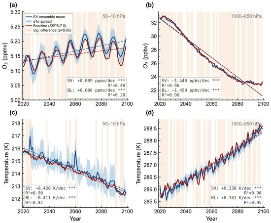
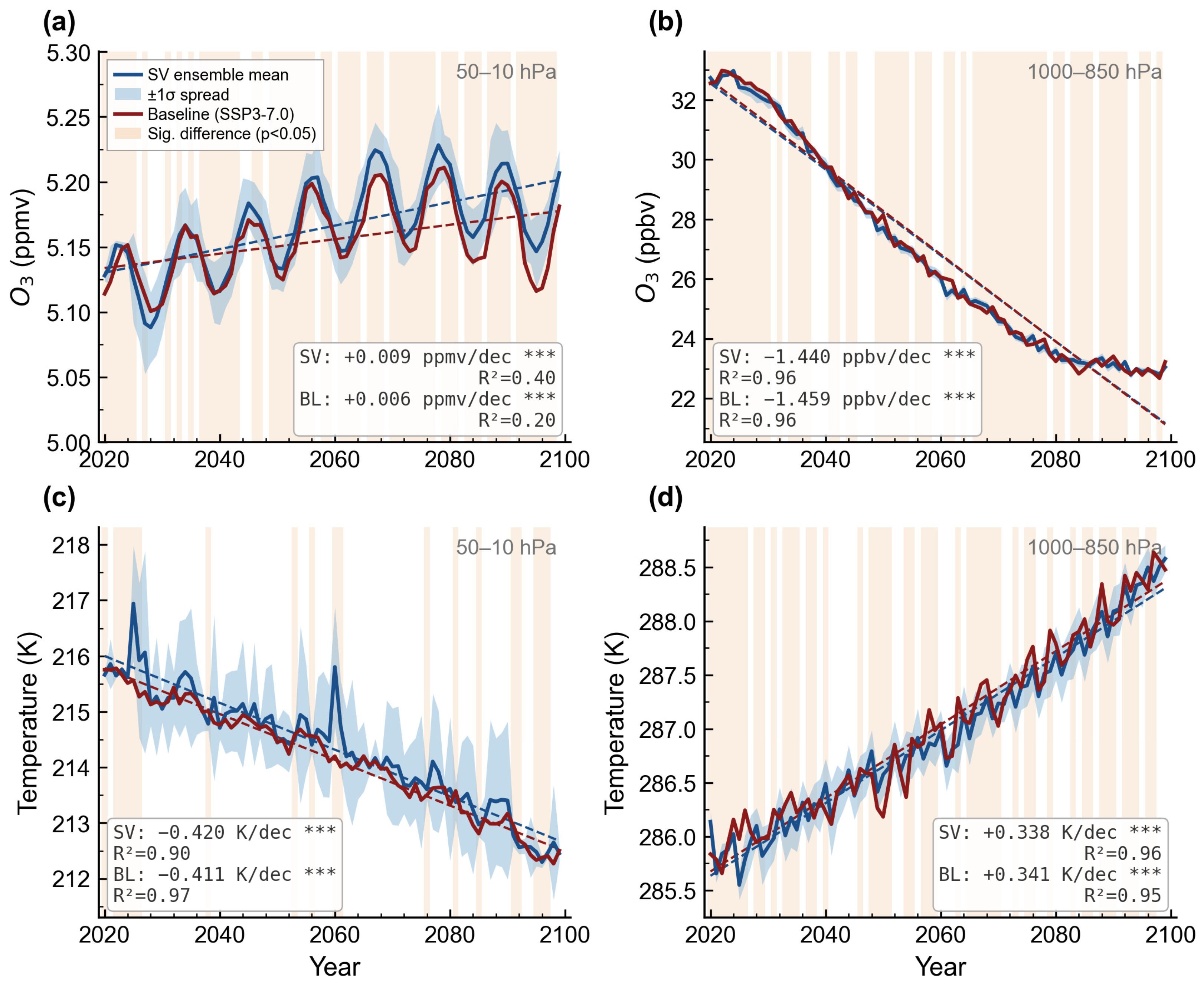
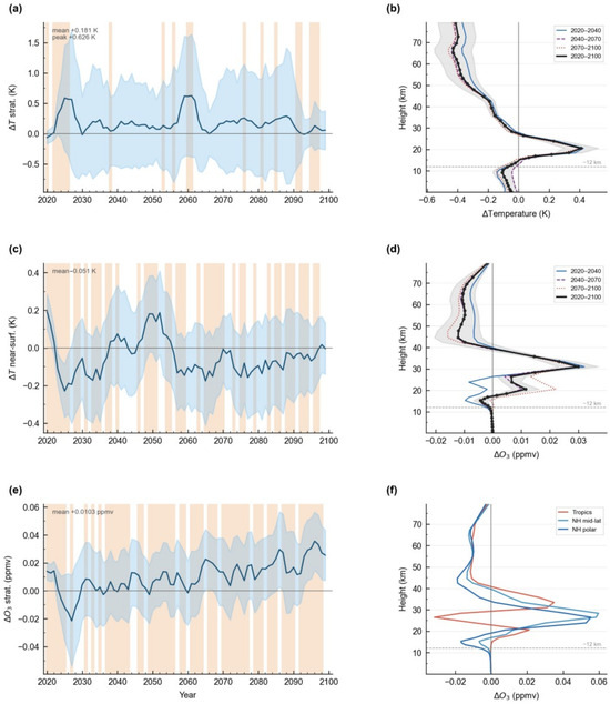
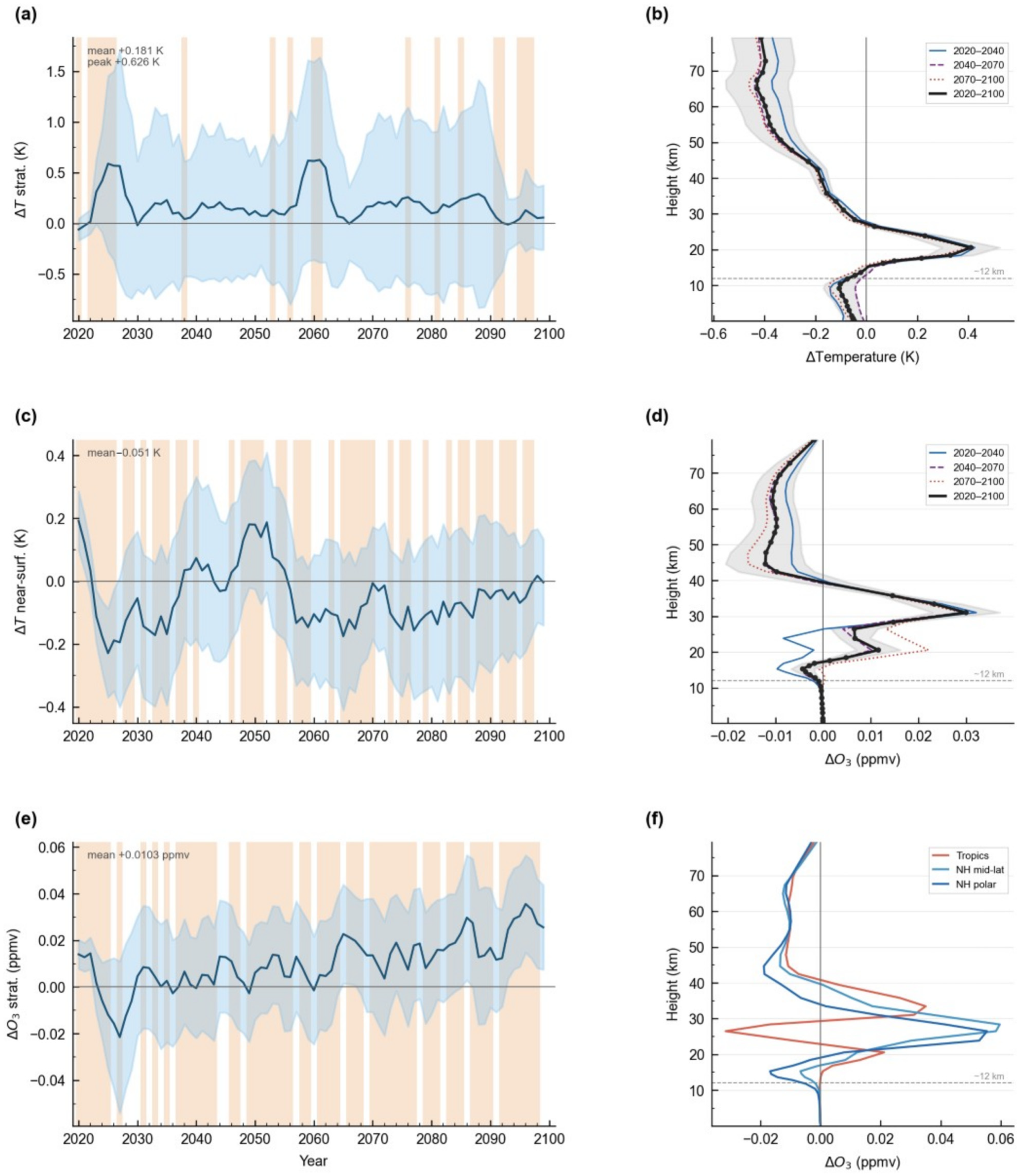
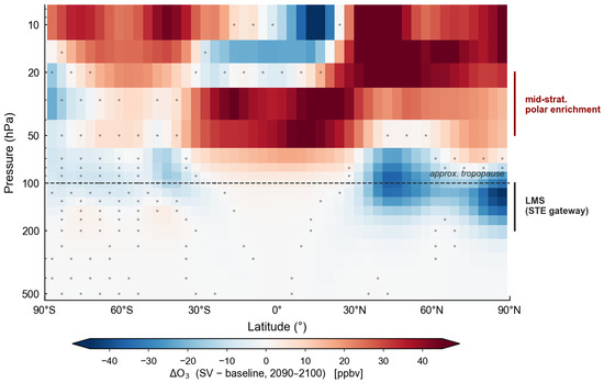
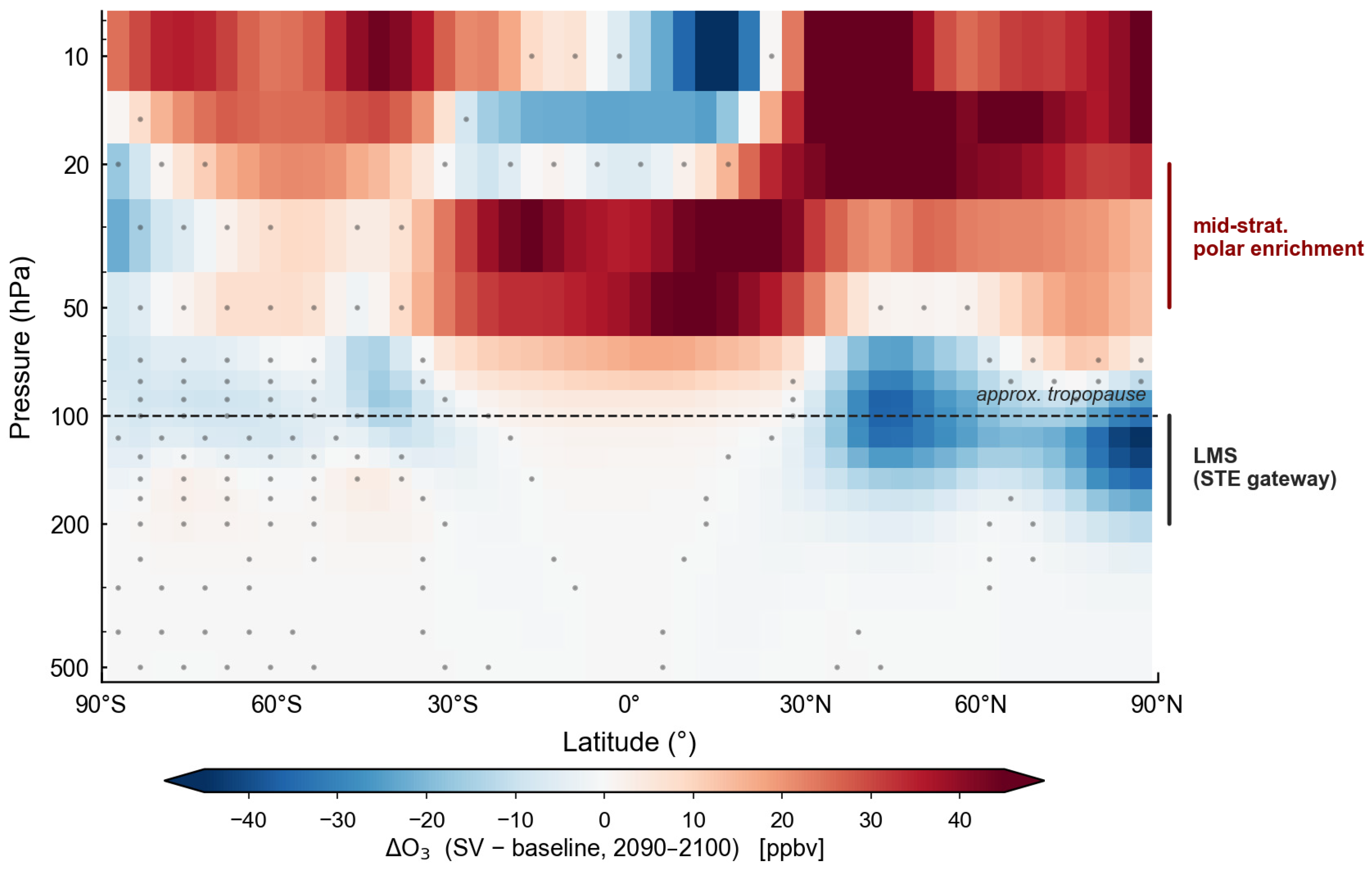
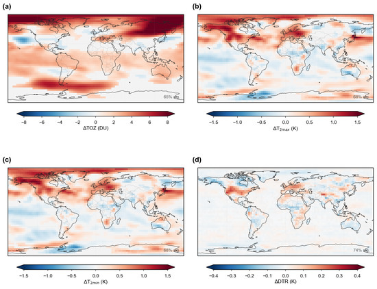
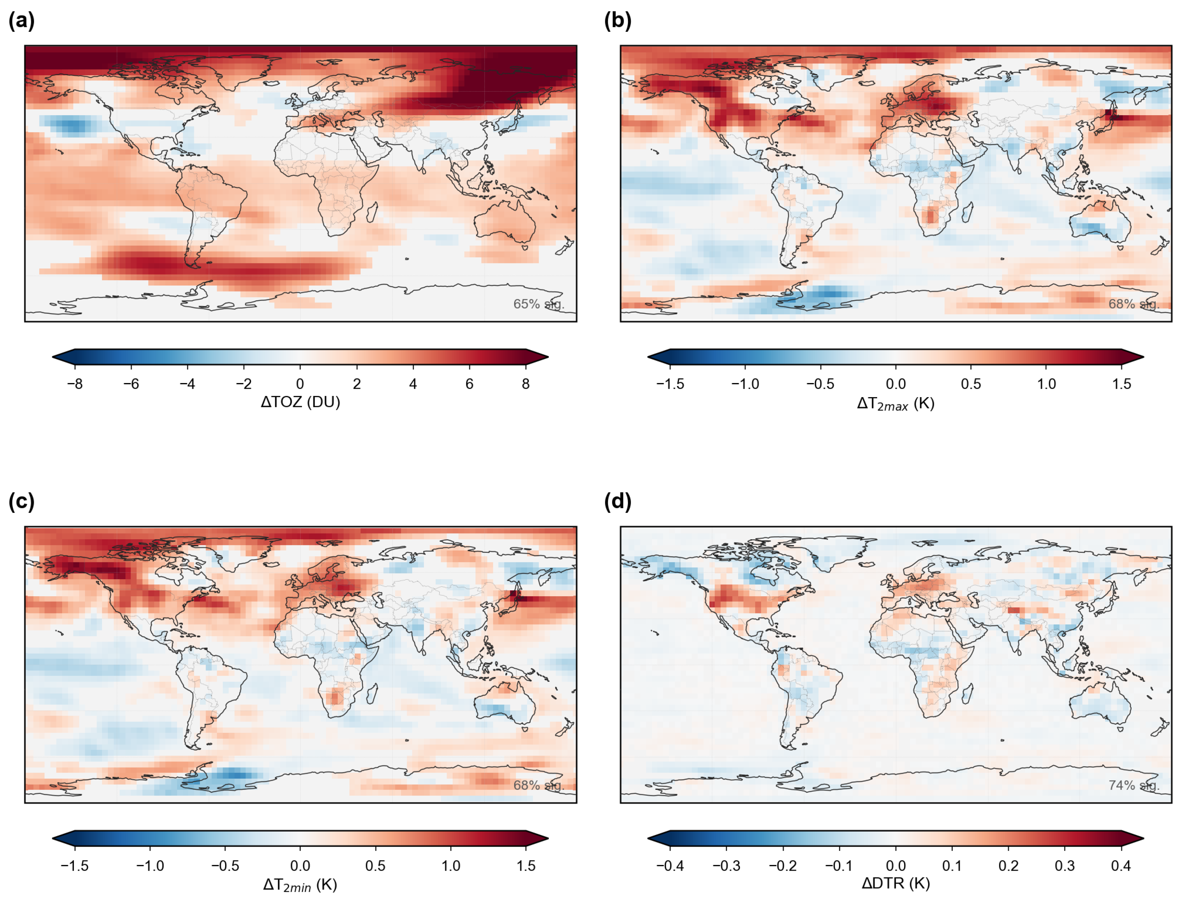
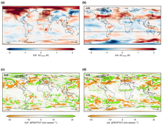
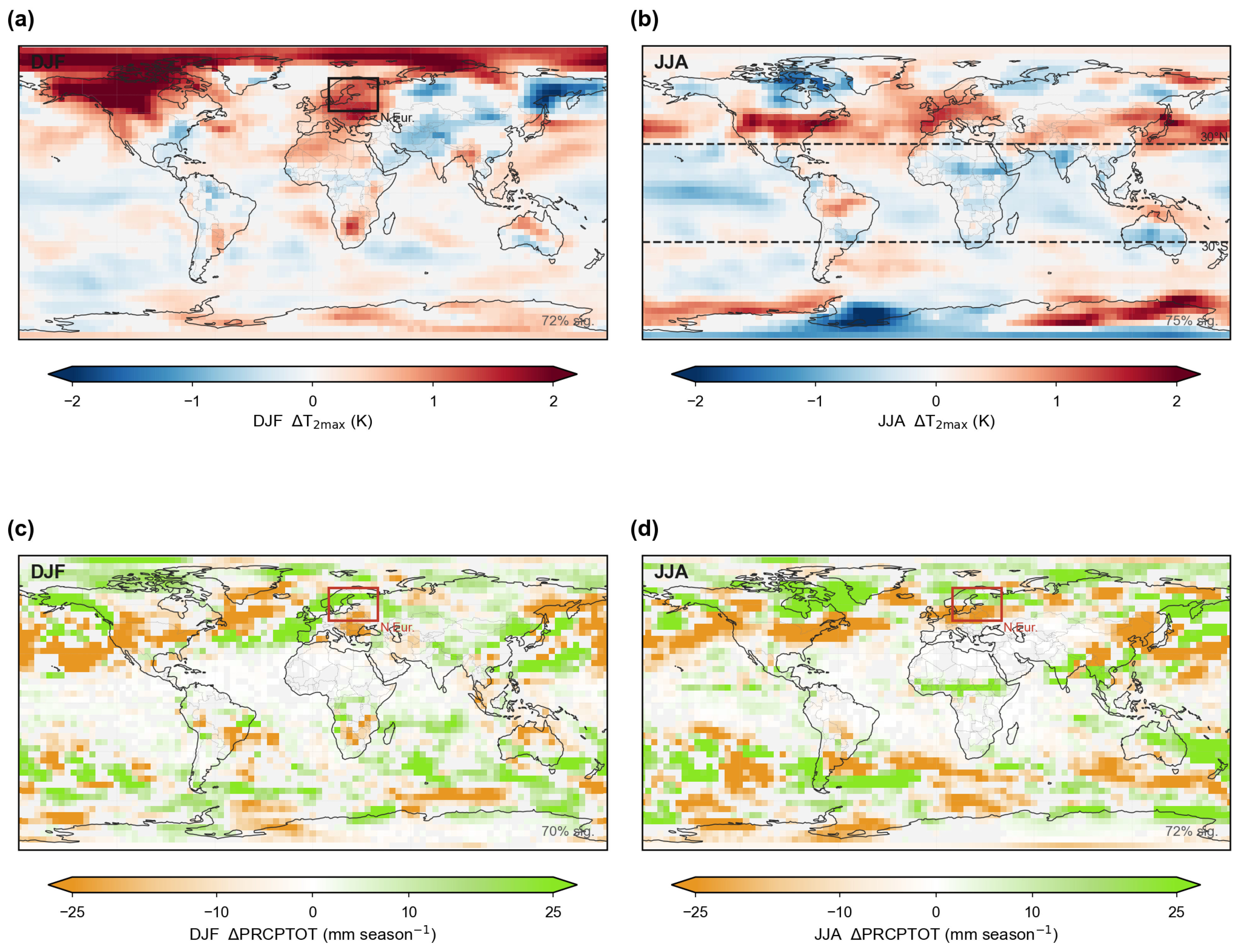
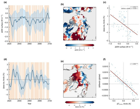
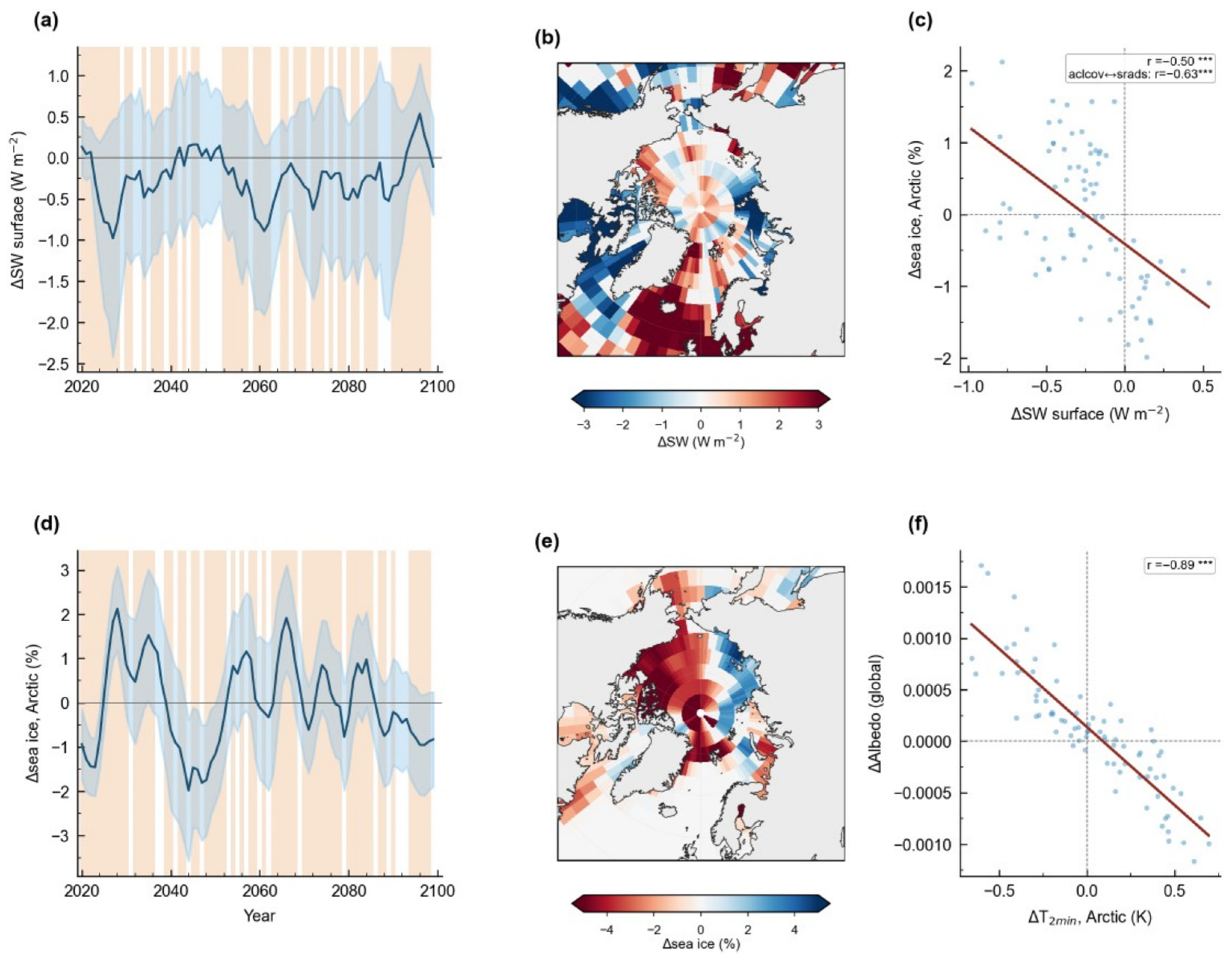
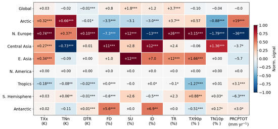
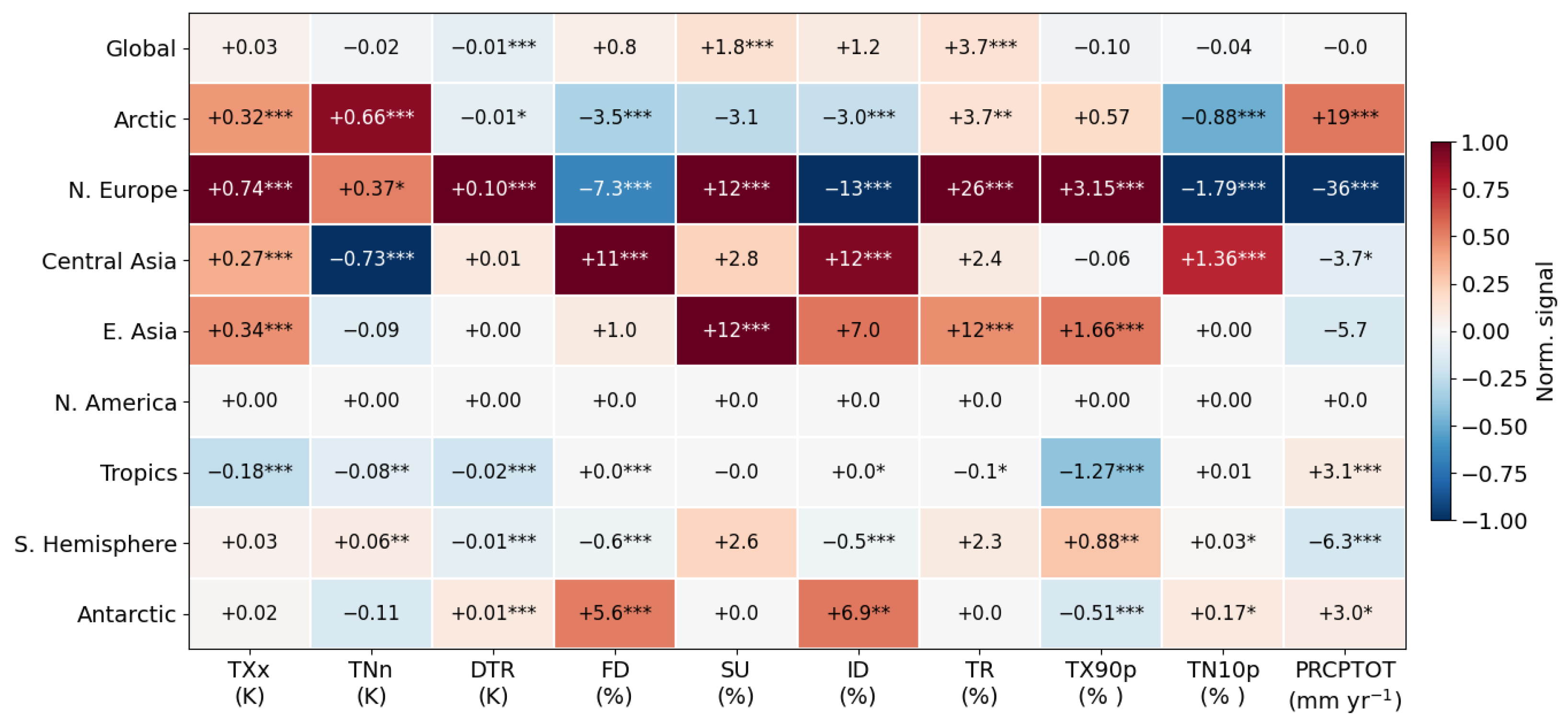
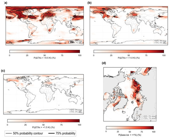
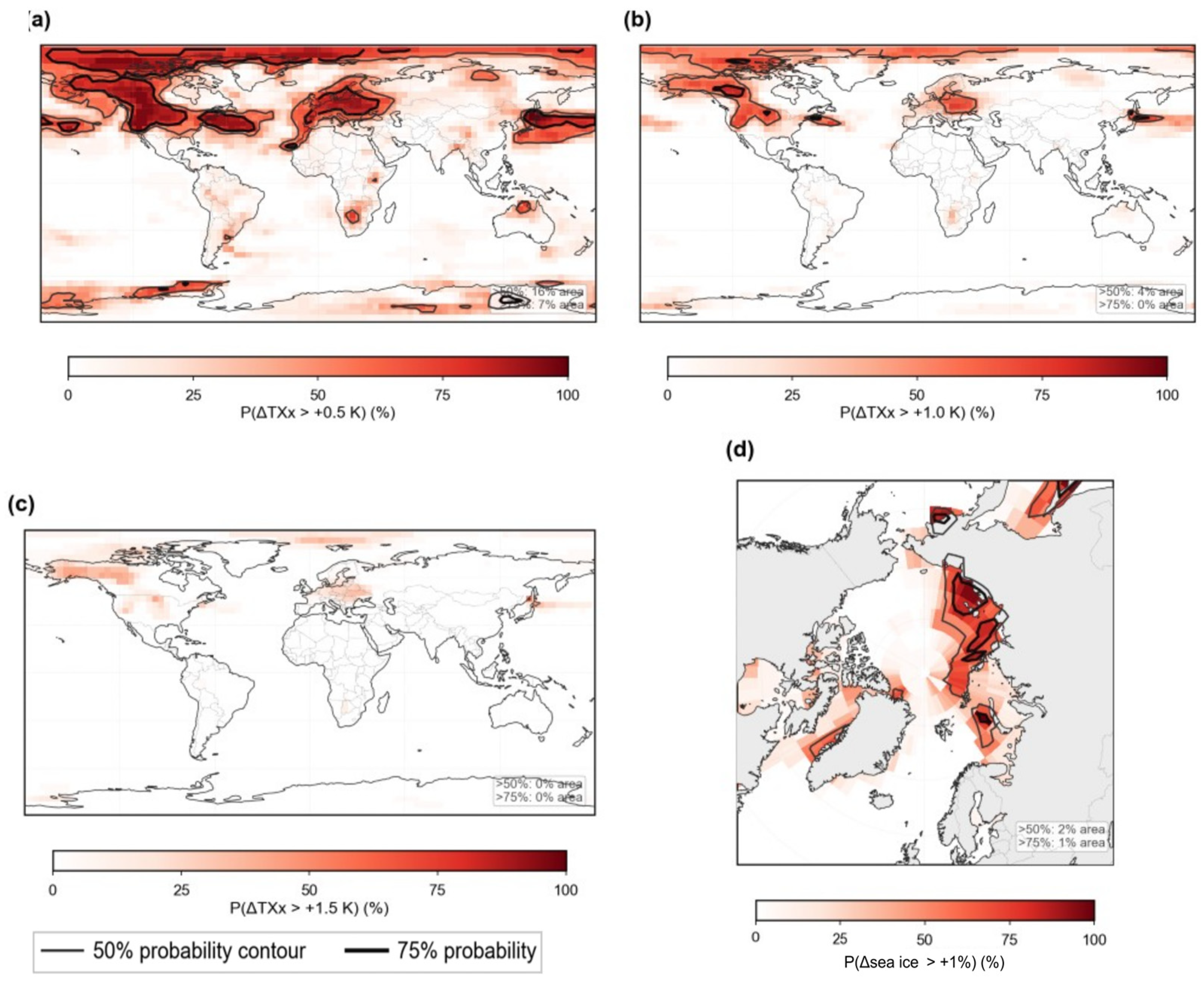
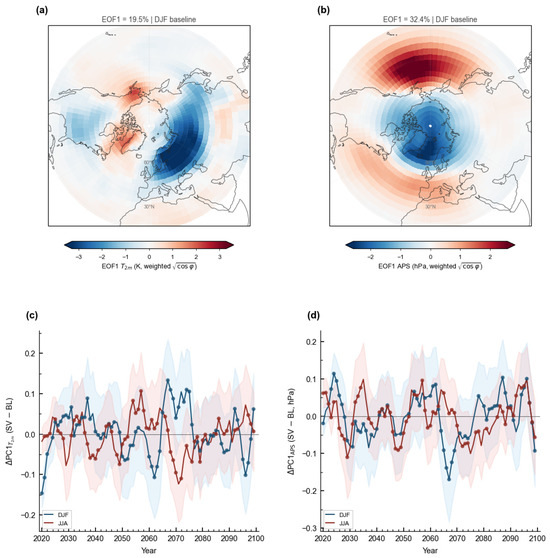
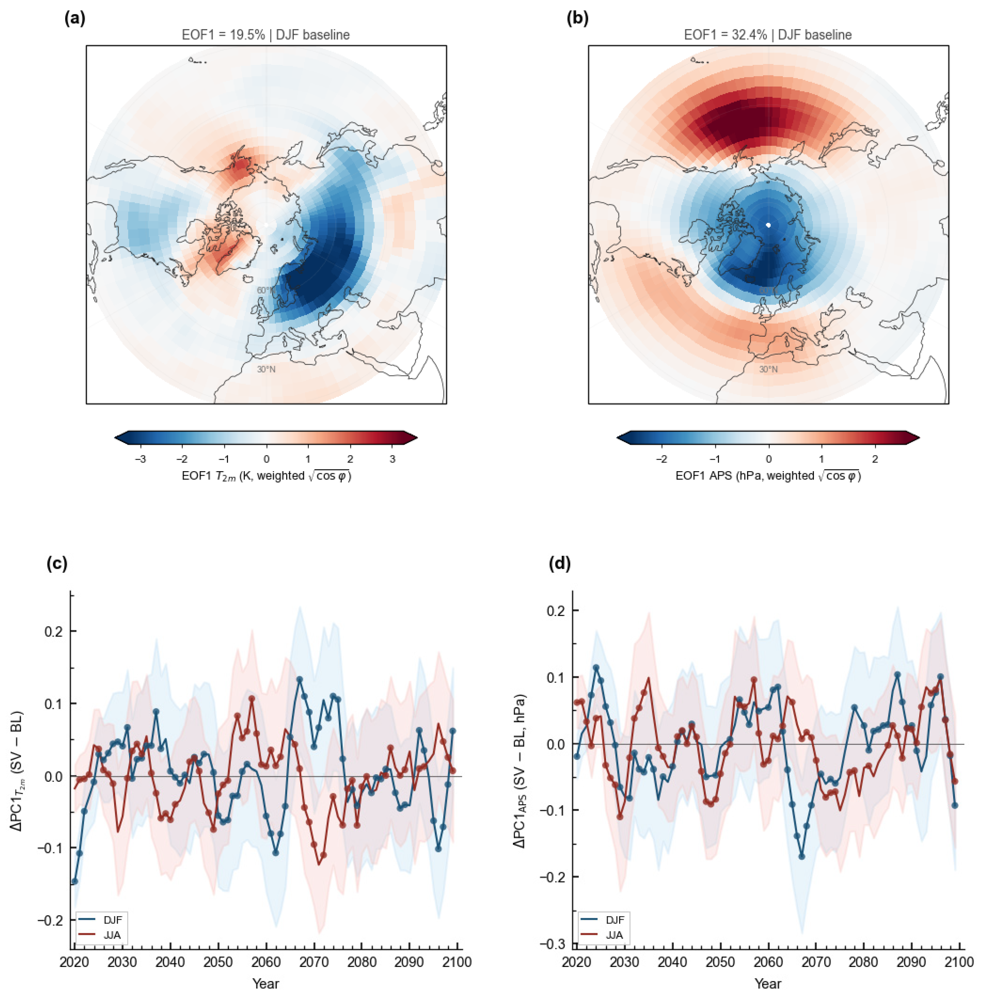

Disclaimer/Publisher’s Note: The statements, opinions and data contained in all publications are solely those of the individual author(s) and contributor(s) and not of MDPI and/or the editor(s). MDPI and/or the editor(s) disclaim responsibility for any injury to people or property resulting from any ideas, methods, instructions or products referred to in the content. |
© 2026 by the authors. Licensee MDPI, Basel, Switzerland. This article is an open access article distributed under the terms and conditions of the Creative Commons Attribution (CC BY) license.