Effects of the Geomagnetic Storm on the Ionosphere on 1 January 2025: A Comparative Analysis of Data from Learmonth and Wake Island

Abstract

This study investigates the ionospheric response in the Southern and Northern Hemispheres over the period from 25 December 2024 to 7 January 2025. A major geomagnetic storm occurred on 1 January 2025, following the consecutive solar wind eruptions on 29–31 December 2024 and 1 January 2025. Global geomagnetic activity monitoring data showed that the Kp index surged to 8+, indicating the occurrence of this major geomagnetic storm. By analyzing the ionosonde, GNSS-TEC, and satellite in situ detection data from Learmonth, Australia (−21.8° N, 114.1° E), as well as Wake Island (19.29° N, 166.65° E), we found that the ionospheric anomalies in the two regions exhibited different patterns. The ionospheric parameters in Learmonth changed much more severely than those in Wake Island in the Pacific region. Relative to normal conditions, the disturbed ionosphere over Learmonth during 1–3 January 2025 exhibited a strong negative storm phase: f_oF₂ decreased by 31.4%, TEC dropped by 27.17%, and M3000F₂ declined by 41.2%, while h_mF₂ increased by 5.2%. This work provides an analysis of the differences in the ionosphere between the Northern and Southern Hemispheres affected by geomagnetic storms in late 2024. These findings highlight the need to incorporate hemispheric asymmetry into ionospheric dynamics models.

1. Introduction

Space weather has profound implications for Earth and other parts of the solar system. The energy core of the solar system is the sun, which is also a major driver for space weather. It continuously transports energy through persistent release of electromagnetic radiation, charged particle streams, and magnetic fields that not only shape Earth’s ionosphere and magnetosphere, but also drive its complex dynamical processes [1]. In the various phenomena related to space weather, the geomagnetic storm phenomenon focused on is a violent disturbance caused by solar wind energy input into the magnetosphere–ionosphere–thermosphere system. This disturbance further influences the ionosphere structure and dynamics by altering the magnetic field of the Earth [2]. Geomagnetic storms have significant effects on the weather and the composition of the upper atmosphere, such as Total Electron Content (TEC). As a key indicator of ionospheric conditions, TEC reflects dynamic changes in electron density during geomagnetic storms. Therefore, analytical studies are necessary to better understand the mechanisms of ionospheric disturbances resulting from geomagnetic storms.

The solar flare is a relatively intense and localized emission of electromagnetic radiation (such as X-rays and ultraviolet rays) in a short period of time, often accompanied by the release of high-energy particles. They usually occur in areas with intense activity and are associated with sunspot phenomena [3]. Based on the X-ray brightness of solar flares in the wavelength range of 1 to 8 Å, they are roughly divided into classes X, M, C, and B [4]. X-class flares are major events (ten times brighter than M-class flares). M-class flares are of medium size (ten times brighter than C-class flares) [5]. C-class and B-class flares are respectively 100 and 1000 times smaller than X-class flares [6].

It is crucial to study the connection between the magnetosphere of the Earth and intense solar activity, which typically occurs during geomagnetic storms and solar flares. Solar flares are produced in the dynamic regions of the Sun, typically adjacent to intricate sunspot configurations, and can last from several minutes to several hours. As the most intense and sudden explosive events on the Sun, these phenomena release torrents of high-energy protons, electrons, and X-ray radiation, which propagate through space and disrupt the plasma equilibrium of the ionosphere. In another scenario, temporal disturbances of the ground magnetic field result from the large-scale solar wind interaction, leading to the changes in the ground ionosphere and subsequently causing the geomagnetic storms to occur [7].

Decades of research have established geomagnetic storms as a key space weather phenomenon [8,9,10]. Geomagnetic storms are disturbances in Earth’s magnetic field that can disrupt technological infrastructure, particularly in telecommunications applications, such as interference with the Global Navigation Satellite System (GNSS) [11,12]. Under the influence of geomagnetic storms, the atmospheric density around satellite orbits increases, leading to greater drag force. As a result, the velocity and altitude of satellites decrease, making it more difficult to maintain their original orbits. Additionally, shortwave communication relies heavily on the ionosphere. During geomagnetic storms, the distribution of electron density changes significantly, leading to variations in the reflection rates of radio waves at different frequencies and causing abnormal reflections of higher-frequency radio waves. If shortwave signals are propagated under these conditions, the signals received at the original reception points will be greatly weakened or completely lost, leading to the cessation of shortwave communication. Therefore, the study of ionosphere disturbances during geomagnetic storms is essential. However, the detailed effects of the ionosphere on various geomagnetic storms and the underlying physical mechanisms remain insufficiently studied [13].

For decades, studies on the ionosphere under geomagnetic storm conditions have been conducted across diverse geographic coordinates, employing both observational data and theoretical frameworks [14,15,16,17,18,19]. According to the concepts proposed by [20,21], the occurrence of geomagnetic storms is due to the solar wind energy being transferred to the space around Earth, leading to dynamic interactions. Such major geomagnetic events can trigger severe damage [22,23]. Energy is injected into the polar regions of Earth. Subsequently, this energy is transferred to the upper atmosphere, generating heat that propagates toward equatorial regions. Ionospheric electron density may fluctuate, either diminishing, amplifying, or remaining stable, depending on whether the storms are driven by CME and CIR. Ionospheric storms manifest in two primary forms: positive and negative. Specifically, parameters such as the ionospheric electron density (Ne), peak electron density (NmF2), and TEC may deviate significantly upward or downward from their nominal quiet-day levels and are corresponding to positive or negative ionospheric storms, respectively.

Statistical analysis of ionospheric storm responses can reveal their seasonal and longitude-related characteristics. These characteristics are well known at middle latitudes. Regarding seasonal differences in thermospheric circulation, summer brings equatorward flows due to both storm-induced and solar-induced circulations, transporting gas with a reduced O/N₂ ratio from the auroral zone to middle latitudes and causing strong negative ionospheric storms. In winter, the opposing circulations lead to an increase in h_mF₂ and corresponding positive ionospheric disturbances. At the same time, equatorward storm-time winds cause ionospheric uplift, making positive storms more easily observed in those regions. Around spring and autumn, negative storms are more common at night in middle and low latitudes. However, for each geomagnetic storm event, the ionospheric response does not perfectly conform to these statistical patterns; it varies significantly with local time, season, and longitudinal/latitudinal dependencies [24]. Longitudinal discrepancies are significant [25]; for example, the geomagnetic dipole offset causes a longitude-dependent balance between solar radiation, electric fields, and neutral winds [26]. The launch of localized gravity waves also plays an important role in the longitudinal dependences [27]. Picanço et al. observed that longitudinal differences during superstorms and the F-region uplifts were influenced by the simultaneity of pre-reversal enhancement (PRE) and electric field penetration [28]. Therefore, case studies of ionospheric storms remain an important approach for understanding the characteristics of storm-time ionospheric responses and their disturbance mechanisms. For typical geomagnetic storm events, a multi-faceted analysis is usually required.

For ionospheric research, several instruments can observe and analyze the characteristics of ionospheric changes from different dimensions. Ionosondes, sounding rockets, incoherent scatter radars, and other observational techniques have been widely used to observe and study ionospheric changes and responses [29,30,31]. However, establishing a dense ionospheric monitoring network remains challenging due to high costs and inaccessible areas. In recent years, multi-frequency or dual-frequency GNSS have become valuable tools for measuring ionospheric TEC and its disturbances [32,33], especially during magnetic storms. Compared with other traditional observational techniques, dense multi-GNSS observational networks can achieve comprehensive coverage and continuous monitoring of the entire ionosphere. GNSS observations provide ionospheric TEC data with high spatial and temporal resolution, which is crucial for correcting ionospheric delay and monitoring space environments [34]. Using GNSS observational data, numerous studies have been conducted on ionospheric changes related to earthquakes, geomagnetic storms, volcanoes, typhoons, and other phenomena [35,36,37,38]. Space physics, geodesy and other fields are particularly focused on using GNSS to study and monitor ionospheric changes [39].

This paper introduces the M-class and X-class solar flares that occurred from late 2024 to early 2025, as well as the major geomagnetic storms during this period, and analyzes the ionospheric changes in two low-latitude regions located in the Southern and Northern Hemispheres with the same absolute values of latitude. The aim is to explore the effect of geomagnetic storms and solar flares on the ionosphere across hemispheres. Although this research is limited to ionospheric data from 25 December to 7 January, it provides valuable insight into how seasonal and geographical differences affect the degree of ionospheric disturbance caused by geomagnetic storms. However, to fully understand the overall ionospheric changes on Earth following solar flares and geomagnetic storms, more ionospheric data from different latitudinal environments are needed, which is key to further in-depth research.

2. Utilization of Data and Employment of Methodology

2.1. Data Sources

In this study, ionospheric parameter data were extracted from the Wake Island station in the Northern Hemisphere and the Australian Learmonth station in the Southern Hemisphere. The data cover the period from 00:00 on 25 December 2024 to 00:00 on 7 January 2025. The data were sourced from the publicly available European ionospheric data in the GIRO Data Center, https://giro.uml.edu/index.html (accessed on 20 May 2025). The parameter variation images were generated using MATLAB software (R2022a). Solar activity monitoring images and analysis charts were obtained from Space Weather Live, https://www.spaceweatherlive.com (accessed on 20 May 2025). Global TEC distribution maps were created based on ionospheric IONEX data from the IGS Data Center, https://igs.org (accessed on 20 May 2025). The Global [O/N₂] ratio was retrieved from the GUVI data (http://guvitimed.jhuapl.edu/data_products) (accessed on 18 May 2026).

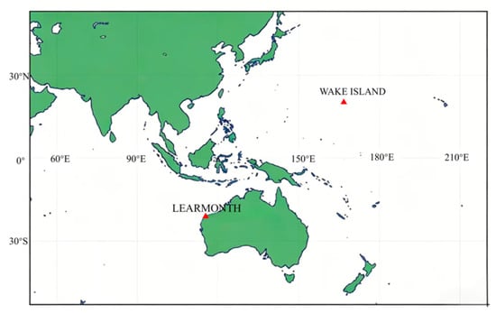
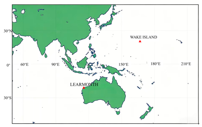
As shown in Figure 1, the two ionosonde stations are located at similar geographic latitudes (~20°) but are different in magnetic latitude: Wake Island (magnetic latitude ~13.65° N) and Learmonth (magnetic latitude ~31.74° S). In addition, the positions of these stations are indicated by red triangles in Figure 1.

Figure 1. The locations of two ionosondes.

2.2. Methodology

TEC is a commonly used parameter to characterize ionospheric plasma density [40]. Slant Total Electron Content (STEC) describes the total amount of free electrons along the line of sight (LOS) of a satellite receiver in the ionosphere. STEC is the number of electrons per m² in a column between the GNSS receiver and the satellite [41]. STEC is defined as follows:

$$\mathrm{STEC}={\displaystyle \frac{1}{40.3}}\left({\displaystyle \frac{f_1^2{f}_2^2}{f_2^2-f_1^2}}\right)(p_1-p_2)$$

(1)

where p₁ and p₂ represent pseudo-ranges with f₁ as 1575.42 MHz and f₂ as 1227.6 MHz frequency, respectively.

STEC can be converted to Vertical Total Electron Content (VTEC) using

$$\mathrm{VTEC}=(\mathrm{STEC}-B_s-B_u)(1-{\displaystyle \frac{{\left(Re\times \cos \epsilon \right)}^2}{{(Re+h)}^2}})$$

(2)

where ε is the angle of the satellite above the horizon; R_e (6371 km) is the average radius of the Earth; B_s and B_u are the equipment biases of satellite and receiver; and h is the height of the ionospheric pierce point. VTEC can be calculated with the specific software [42].

In order to characterize the disturbances of ionospheric TEC, the changing rate of the inclined TEC is calculated. In addition, the Rate of TEC Index (ROTI), considering the average standard deviation of the STEC rate, is also calculated. Irregularities in the ionosphere are obtained through fluctuations in rapidly changing GNSS signals corresponding to TEC. ROT is the difference in the nominal STEC values observed over intervals equal to one minute in selected time units. ROT is measured in TECU/min, which directly represents signal fluctuations caused by the structure of the ionosphere. The ROT expression is given by

$$\mathrm{ROT}={\displaystyle \frac{{\mathrm{STEC}}_{(k+1)}^i-{\mathrm{STEC}}_k^i}{t_{(k+1)}-t_k}}$$

(3)

In the above equation, ${\mathrm{STEC}}_{k+1}^i$ and ${\mathrm{STEC}}_k^i$ represent the STEC at the k + 1 and k time periods, respectively, and i denotes the number of visible satellites. The typical unit for ROT is TECU per minute. Meanwhile, ROTI, calculated as the standard deviation of ROT values, serves to characterize the occurrence of irregularities in ionospheric plasma density, providing correction information for navigation systems to improve positioning accuracy.

ROTI is an indicator that measures the degree of ionospheric disturbances, reflecting the rapid changes of TEC. Therefore, it can be used to predict the dynamic characteristics of the ionosphere. Rapid changes in the ionosphere can cause signal propagation delays in navigation systems, leading to a decrease in positioning accuracy. ROTI can be used to detect and monitor such ionospheric disturbances, providing correction information for navigation systems to improve positioning accuracy.

ROTI is the standard deviation over a certain time interval of ROT, so it is defined as follows:

$$\mathrm{ROTI}=\sqrt{⟨{\mathrm{ROT}}^2⟩-{⟨\mathrm{ROT}⟩}^2}$$

(4)

Solar flares can be divided into A, B, C, M and X intensity categories, depending on peak flux intensity (W/m²) and brightness in the wavelengths of the X-ray [43]. From the end of December 2024 to the beginning of January 2025, the Sun experienced significant activity, with large numbers of X and M class flares occurring.

3. Results

In this work, we investigated the differences in low latitude ionospheric changes between the Southern and Northern Hemispheres during geomagnetic storms caused by intense solar activity. Data from ionosonde stations in Australia and the Pacific were used to determine the causes of these differences.

3.1. Occurrence of Geomagnetic Storms After Intense Solar Activity

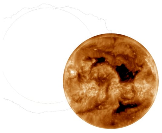
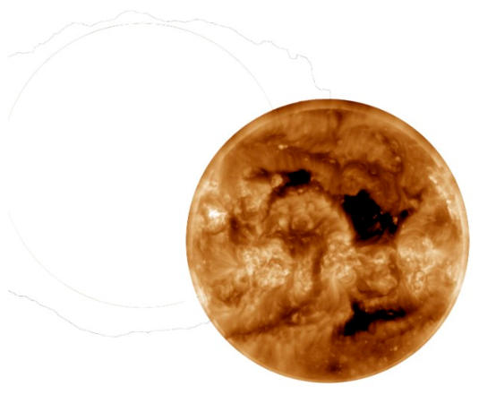
Figure 2 shows the solar surface observation image on 3 January. The image reveals a large number of sunspots on the solar surface that day, with variations in the sunspots being positively related to the intensity of solar activity. When solar activity is strong, a large number of sunspots are produced, and the number of sunspots also increases significantly. Therefore, the observation and analysis of sunspot number, area, distribution, and evolution can well reflect the overall intensity of solar activity and provide an important basis for the prediction and study of solar activity.

Figure 2. Large sunspot region on the solar surface on 3 January.

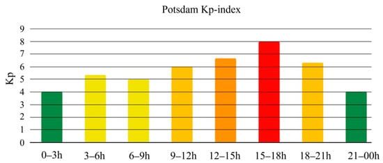
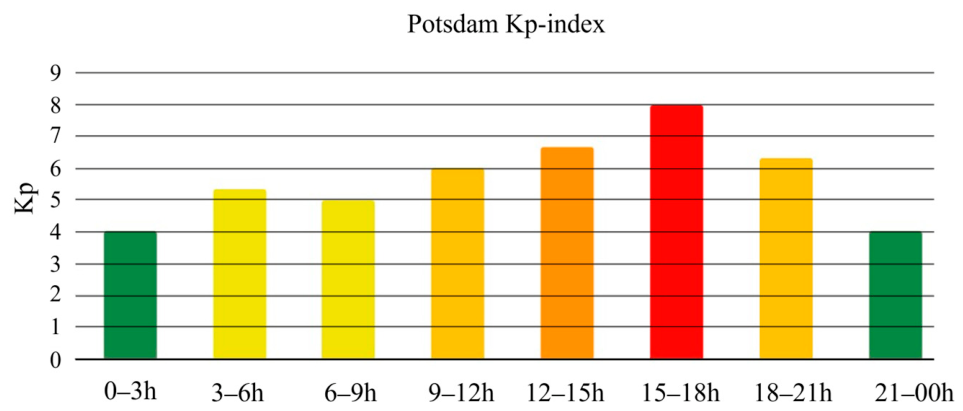
Figure 3 shows that after a series of intense solar activities began at the end of December, a strong geomagnetic storm was triggered on 1 January. According to measurements from geomagnetic observatories, the geomagnetic data reached above level 8 between 15:00 and 18:00.

Figure 3. Abnormal Earth Kp index values on 1 January, with an intense geomagnetic storm from 15:00 to 18:00, Kp values use a diverging color scale: green (quiet) through yellow/orange to red (intense storm, Kp ≥ 7).

3.2. Solar Activity Intensity and Earth Monitored Kp Index Values

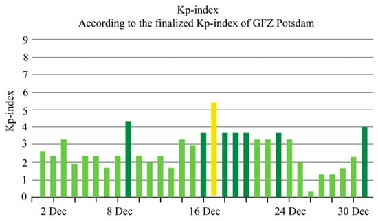
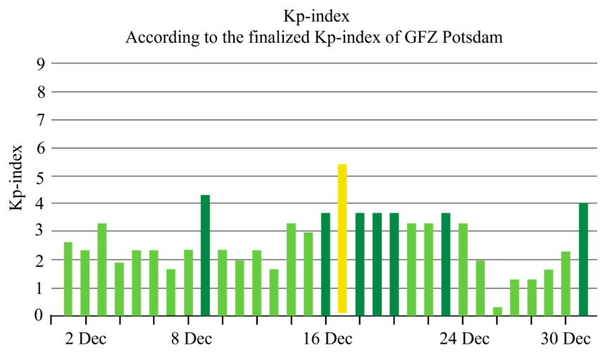
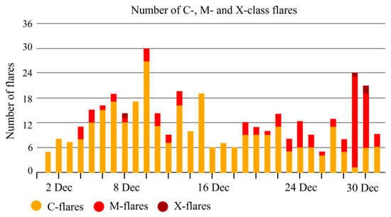
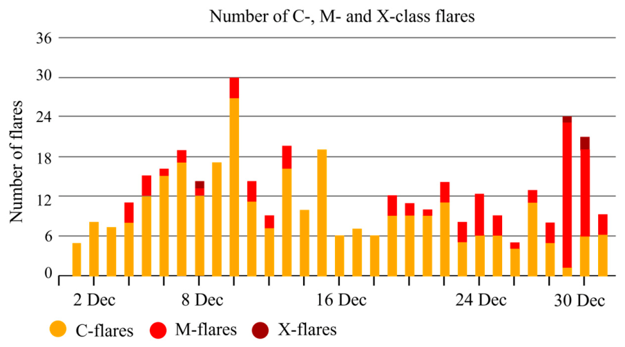
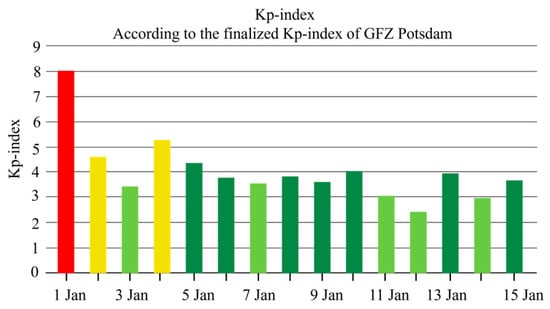
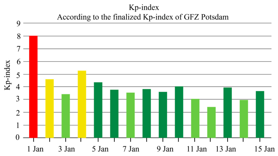
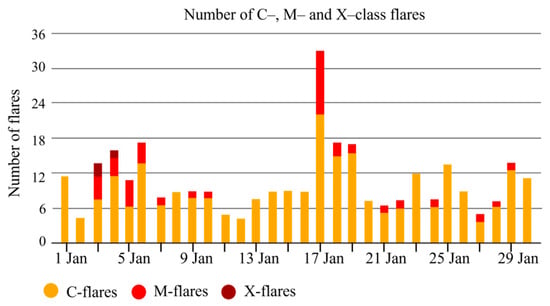
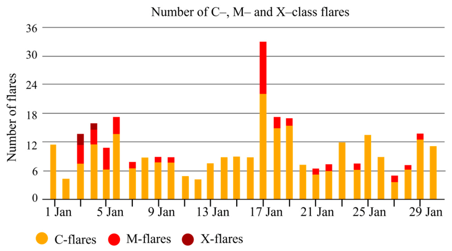
Figure 4, Figure 5, Figure 6 and Figure 7 show that solar activity became intense after 28 December, with many M-class flares and a few higher-energy X-class flares occurring, finally triggering an extremely strong geomagnetic storm on 1 January 2025.

Figure 4. Changes in Earth Kp index in December 2024. Kp values use a diverging color scale: green (quiet) through yellow (moderate storm).

Figure 5. Changes in solar activity intensity in December 2024. The histogram depicts the frequency of solar flares categorized by class C-class flares in orange, M in red, X in brown.

Figure 6. Changes in Earth Kp index in January 2025. Kp values use a diverging color scale: green (quiet) through yellow/orange to red (intense storm, Kp ≥ 7).

Figure 7. Changes in solar activity intensity in January 2025. The histogram depicts the frequency of solar flares categorized by class C-class flares in orange, M in red, X in brown.

3.3. Global Ionospheric TEC Variations

From the end of December to the beginning of January, the Northern Hemisphere is in winter, receiving less solar energy, and thus TEC values are generally low. In contrast, the Southern Hemisphere is in summer, with strong solar radiation, resulting in generally higher TEC values. This leads to differences in TEC distribution across hemispheres. The impact of geomagnetic storms resulting from solar activity on the ionosphere in the Southern and Northern Hemispheres varies depending on geographical location and season. Studying the ionosphere TEC of Southern and Northern Hemispheres is of great importance for assessing the impact on communication conditions.

This work used ionosonde data from two locations in different regions: Learmonth in Australia in the Southern Hemisphere and Wake Island in the Northern Hemisphere. The absolute values of the latitudes of these two locations are the same, eliminating the influence of latitude differences on the ionosphere. The changes in ionospheric parameters during geomagnetic storms were obtained by analyzing the variation in ionospheric parameters from 25 December to 7 January.

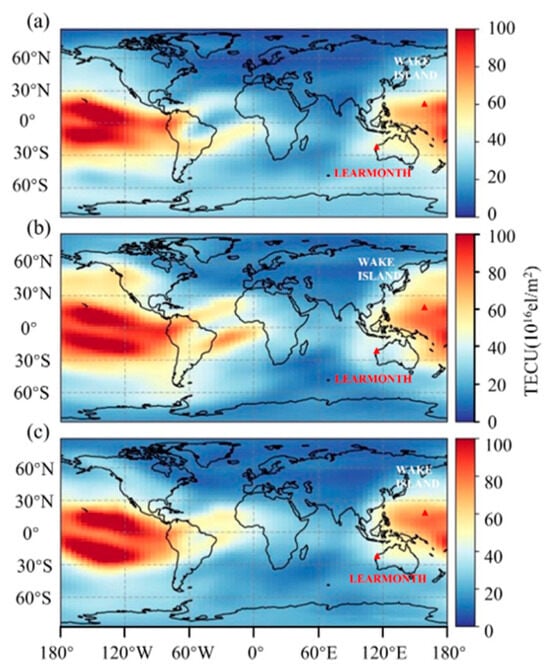
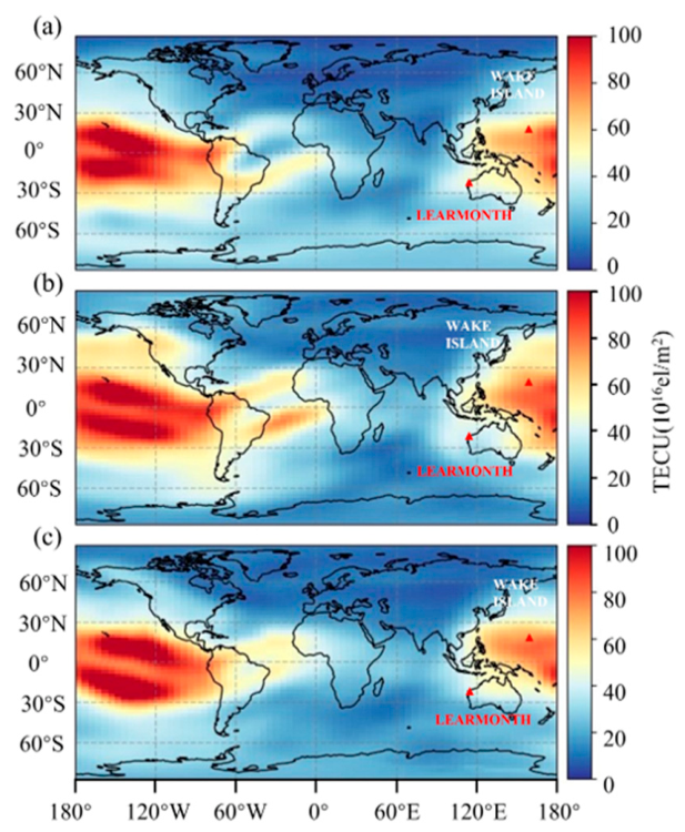
After data analysis, it was found that during the above observations, the ionosphere in the Southern Hemisphere underwent significant changes, while the ionosphere in the Northern Hemisphere changed less. This confirms that solar flares have a significant effect on ionosphere, with cross-hemispheric differences due to seasonal variations. The following figures show the global ionospheric TEC distribution maps at 00:00 on 26 December, 1 January, and 5 January, illustrating the global ionospheric TEC distribution before, during, and after the geomagnetic storm.

As shown in Figure 8, the global Total Electron Content (TEC) map reveals a significant longitude asymmetry during the geomagnetic storm of 1 January 2025. The Learmonth region in the Southern Hemisphere experiences a large-scale decrease in TEC compared to the normal TEC distribution map on 26 December. After the geomagnetic storm ended on 5 January, the TEC in the Learmonth region recovered significantly, and the ionospheric environment returned to normal. No substantial changes were seen in Wake Island throughout the storm period.

Figure 8. Global TEC changes (a) before the geomagnetic storm on 26 December, (b) during the geomagnetic storm on 1 January, and (c) after the geomagnetic storm ended on 5 January.

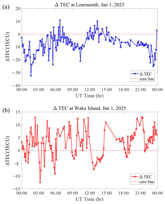
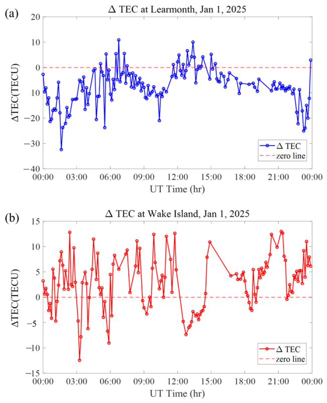
Figure 9 shows the TEC difference relative to the quiet day (ΔTEC) over Learmonth and Wake Island on 1 January 2025. Figure 9a shows that ΔTEC at Learmonth stayed below the zero line for almost the full storm time, reaching a minimum of about −30 TECU around 03:00 UT. Figure 9b shows the ΔTEC at Wake Island, which frequently oscillated near the zero line. At Wake Island, the background average TEC was about 37 TECU, making the ±10 TECU fluctuations relatively small (about 30% of the background value). In contrast, at Learmonth, the background average TEC was only about 7 TECU. Although the absolute ΔTEC values at Learmonth appear smaller, they represent larger relative changes (~200% of the background), indicating a more severe ionospheric disturbance compared to its quiet-time baseline. Accordingly, Learmonth experienced a significantly stronger storm than Wake Island.

Figure 9. The TEC difference relative to the quiet day (ΔTEC) over (a) Learmonth station and (b) Wake Island station, 00:00–24:00 UT on 1 January 2025.

3.4. Variations on Wake Island from 25 December 2024 to 7 January 2025

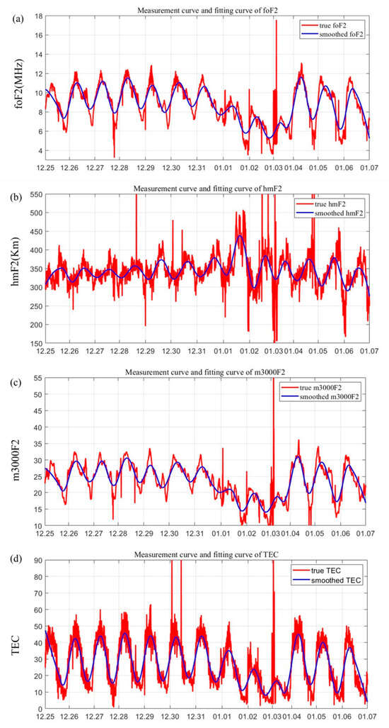
Further analysis was conducted on the ionosonde data from specific regions. Ionospheric data from the ionosonde stations on Wake Island in the Pacific and Learmonth in Australia were used. The parameters analyzed included f_oF₂, h_mF₂, M3000F₂, and TEC. Curves were plotted using the measured data from 25 December 2024 to 7 January 2025, and the trends were analyzed by fitting curves.

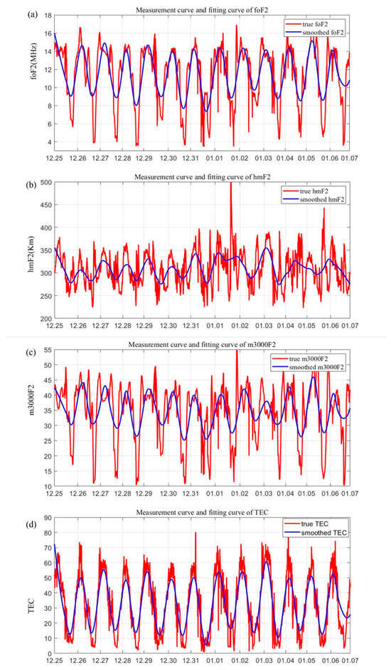
Figure 10 shows the ionospheric parameter variations on Wake Island from 25 December to 7 January. During this geomagnetic storm, the parameters on Wake Island did not show any significant anomalies in terms of numerical values.

Figure 10. Changes in ionospheric parameters on Wake Island from 25 December to 7 January: (a) f_oF₂, (b) h_mF₂, (c) M3000F₂ and (d) TEC.

Table 1 shows the median values of ionospheric parameters in Wake Island in the Northern Hemisphere from 25 December 2024 to 6 January 2025. The analysis indicates that the occurrence of the geomagnetic storm did not have a major influence on the ionospheric parameters at the same latitude in the Northern Hemisphere, and the ionospheric parameters remained consistent with the normal state.

Table 1. Daily median values of ionospheric parameters at Wake Island in the Pacific.

Date	foF2	M3000F2	hmF2	TEC
25 December 2024	13.375	39.22	304.6	37.6
26 December 2024	13.15	41.38	298.5	30.4
27 December 2024	12.95	38.75	299.3	31.3
28 December 2024	12.2	36.85	297.7	34.3
29 December 2024	12.5	38.73	304.4	32.9
30 December 2024	12.4625	36.96	303.6	31.65
31 December 2024	11.625	34.71	321.4	25.6
01 January 2025	12.95	36.385	331.75	37.85
02 January 2025	13.0065	38.08	308.05	30.5
03 January 2025	12.5625	34.385	301	28.05
04 January 2025	11.45	34.84	316	29.4
05 January 2025	13.375	38.42	308.7	33.5
06 January 2025	12.413	36.54	302.3	30.1

3.5. Ionospheric Parameter Variations in Australia from 25 December 2024 to 7 January 2025

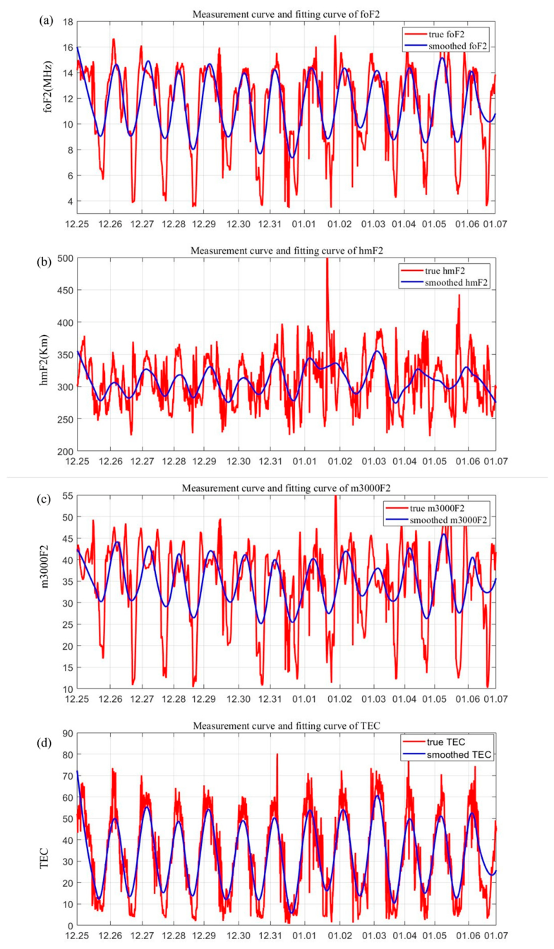
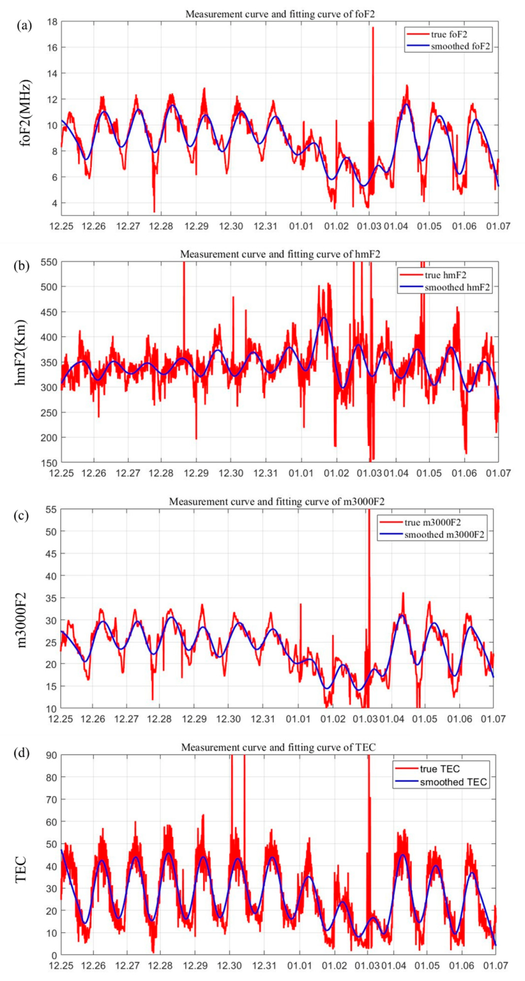
Figure 11 shows the ionospheric parameter variations in Learmonth from 25 December to 7 January. Under the influence of this geomagnetic storm, f_oF₂, M3000F₂, and TEC decreased sharply, while h_mF₂ increased compared to the normal state.

Figure 11. Changes in ionospheric parameters in Australia from 25 December to 7 January: (a) f_oF₂, (b) h_mF₂, (c) M3000F₂ and (d) TEC.

Table 2 shows that from 25 December 2024 to 6 January 2025, the ionospheric parameters in the Learmonth region of the Southern Hemisphere changed significantly. The f_oF₂ parameter decreased by 31.4% compared to the normal state, M3000F₂ decreased by 41.2%, h_mF₂ increased by 5.2%, and TEC decreased by 27.17%. It is concluded that during this geomagnetic storm, the ionospheric parameters in the Southern Hemisphere changed dramatically, while the ionospheric parameters in the Northern Hemisphere did not show significant fluctuations.

Table 2. Daily median values of ionospheric parameters in the Learmonth region of Australia.

Date	foF2	M3000F2	hmF2	TEC
25 December 2024	24.405	27.3	331.6	8.9875
26 December 2024	27.005	29.5	332.2	9.8875
27 December 2024	26.96	32.85	337.7	9.65
28 December 2024	27.56	30.3	343.5	10.225
29 December 2024	24.465	28.85	343.65	9
30 December 2024	26.69	29.5	346.05	10.075
31 December 2024	24.98	27.5	350.8	9.3
01 January 2025	18.06	22.4	372.2	7.6
02 January 2025	17.52	14	341.5	6.675
03 January 2025	17.79	13.2	356.3	6.525
04 January 2025	27.39	30.9	338.6	9.8
05 January 2025	26.11	25	338.2	9.7
06 January 2025	23.77	19.6	326.1	8.575

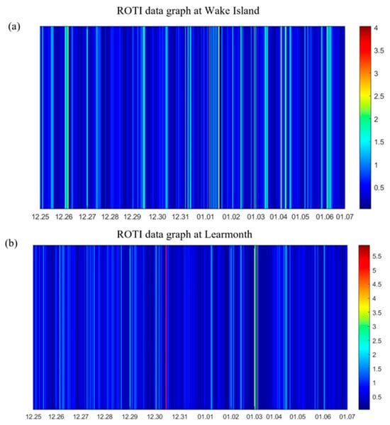
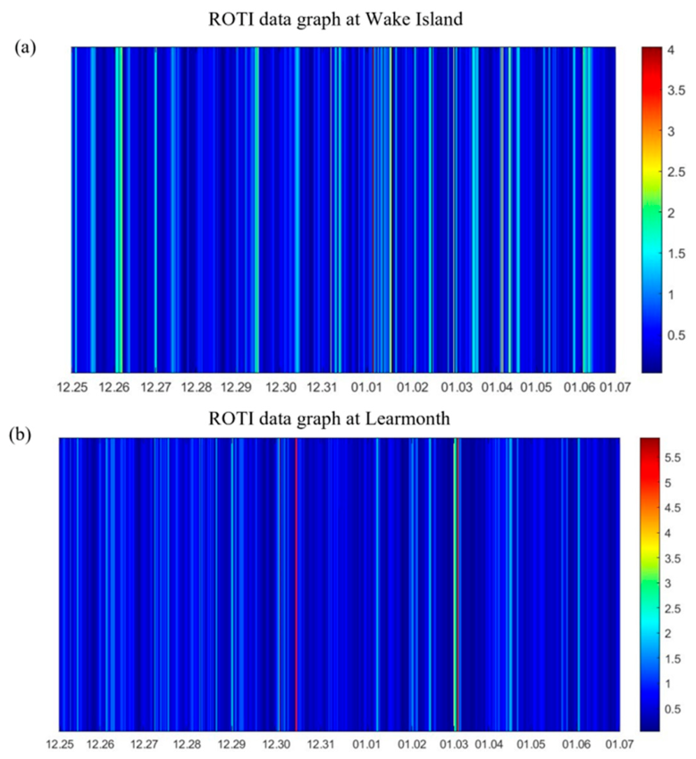
Using the TEC Rate of Change Index (ROTI) calculated with a 5 min sliding window, we obtained the temporal variations of ROTI at Learmonth and Wake Island from 25 December to 7 January, as shown in Figure 12. The ROTI reflects the degree of ionospheric disturbance caused by geomagnetic storms.

Figure 12. ROTI parameters of the ionosphere at (a) Wake Island and (b) Learmonth from 25 December 2024 to 7 January 2025.

As shown in Figure 12a, at Wake Island, only a brief TEC fluctuation occurred on the afternoon of 1 January. Since the TEC values did not decrease significantly, the ROTI pattern still exhibited an alternating high and low sequence, similar to normal conditions. In contrast, the ionosphere over Learmonth displayed intense and prolonged ROTI fluctuations starting from 2 January and continuing through 3 January. Moreover, low ROTI values were observed both before and after this fluctuation episode, indicating relatively calm conditions, while the intense fluctuations during the episode reflect strong TEC variations associated with the storm. These observations are consistent with Learmonth’s ionospheric TEC monitoring data under geomagnetic storm conditions.

4. Discussion

4.1. Spatial Distribution of [O/N₂] During Quiet and Disturbed Conditions

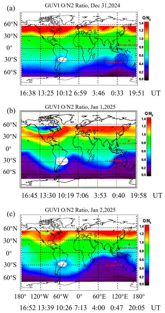
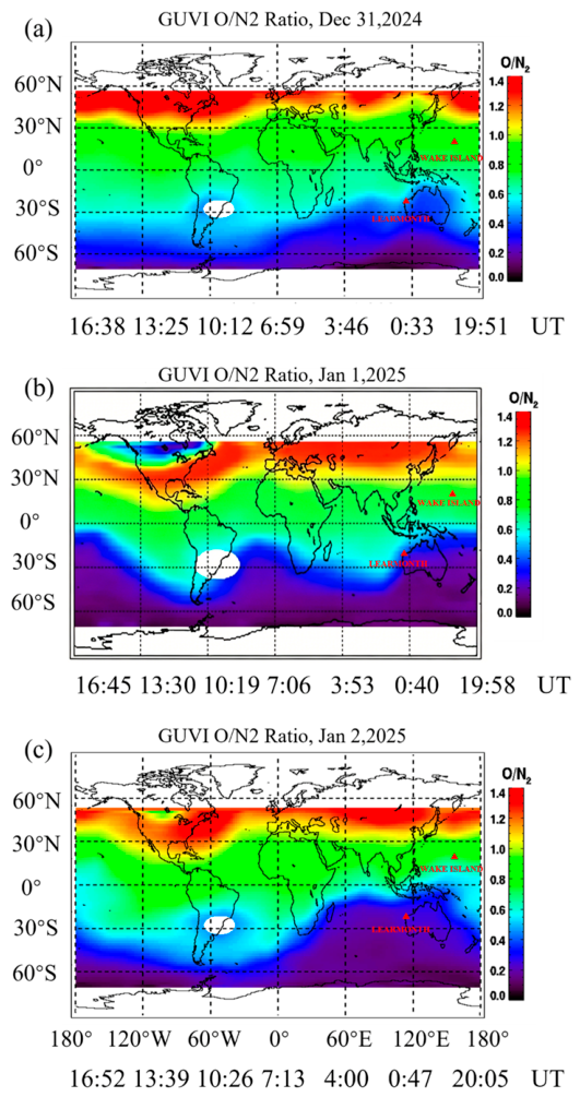
To evaluate the storm’s impact on thermospheric composition at two specific sites, we compared the [O/N₂] ratio observed at Learmonth and Wake Island under geomagnetically quiet and disturbed conditions, as shown in Figure 13. On the quiet day, both sites exhibited similar and stable [O/N₂] values, with Learmonth consistently lower than Wake Island due to the seasonal background. During the storm, however, the two sites showed different behaviors. At Learmonth, the [O/N₂] ratio displayed a large fluctuation and a significant downward trend, reflecting strong storm-enhanced circulation and unevenly redistributed atomic oxygen and molecular nitrogen reaching this region. In contrast, at Wake Island, the [O/N₂] ratio remained relatively stable with only minor variations throughout the storm time, suggesting a much weaker thermospheric response. This contrasting behavior implies an asymmetric interhemispheric effect of the geomagnetic storm, which may be further modulated by longitudinal differences in storm-enhanced circulation and energy deposition. Specifically, the propagation of storm-enhanced disturbances toward Learmonth was enhanced, while Wake Island remained comparatively sheltered.

Figure 13. Daily variation in [O/N₂] ratio from GUVI on (a) 31 December 2024, (b) 1 January 2025 and (c) 2 January 2025.

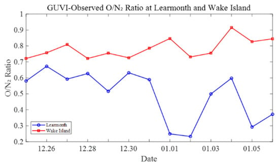
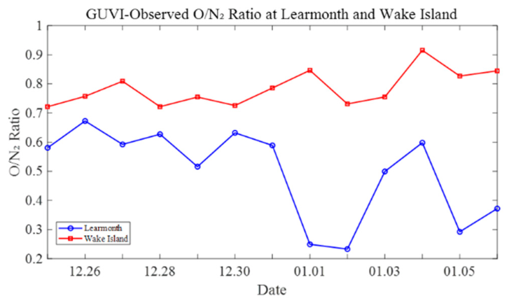
As shown in Figure 14, The time series clearly illustrates a significant asymmetric response in the thermospheric O/N₂ ratio between Learmonth and Wake Island during the geomagnetic storm in early January 2025. Prior to the storm (26–31 December), Learmonth exhibited a relatively stable O/N₂ baseline near 0.6, while Wake Island maintained a higher baseline around 0.8. However, as the storm intensified around 1 January, Learmonth dropped sharply from 0.6 to a minimum of 0.25. In contrast, Wake Island remained relatively stable, with its O/N₂ ratio staying high (0.7).

Figure 14. Changes in the thermospheric O/N₂ ratio in Learmonth and Wake Island from 25 December to 6 January.

4.2. Role of the Penetration Electric Field (PPEF)

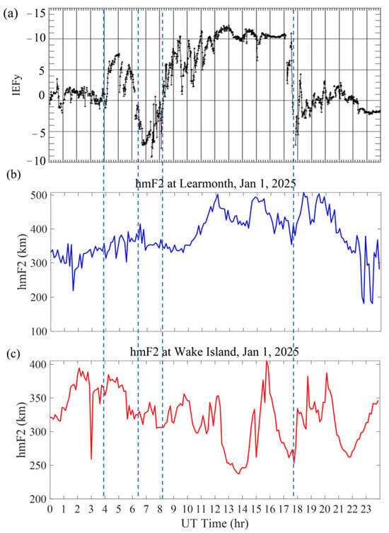
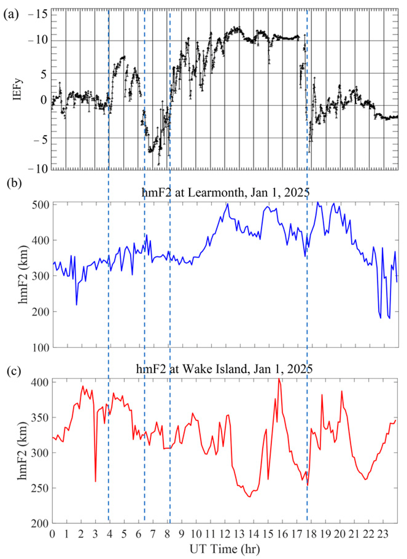
To study the penetration electric field (PPEF) modulation during the storm, we examined the interplanetary electric field IEFy and the h_mF₂ responses at two low-latitude stations. IEFy values were obtained from the Space Physics Data Facility (SPDF) at http://omniweb.gsfc.nasa.gov/ow_min.html (accessed on 15 May 2026). As shown in Figure 15a, IEFy is positive from 09:00 to 18:00 UT, indicating the presence of a penetrating electric field. Figure 15b,c show the h_mF₂ variations at Learmonth and Wake Island, respectively. At the Learmonth station, h_mF₂ shows a significant corresponding clear uplift when the IEFy was positive. However, at Wake Island, the response of h_mF₂ is more complex; it increases slightly around 11:00 UT, then drops sharply near 14:00 UT, subsequently rises again to a higher altitude between 15:00 and 17:00 UT, and finally decreased at 18:00 UT. The difference in h_mF₂ response between the two sites can be attributed at least in part to the influence of local neutral winds, as outlined by N. Balan et al. [44]. Specifically, at Wake Island, a poleward neutral wind, opposite to the upward E × B drift driven by the penetrating electric field, may have temporarily suppressed F-layer uplift, resulting in a sharp drop in h_mF₂ around 14:00 UTC. In contrast, the positive IEFy at the same time was consistent with the eastward electric field driving the upward E × B drift, as observed at Learmonth. Therefore, while the penetrating electric field remains the primary driver of the overall increase in h_mF₂, neutral winds can modulate the local ionospheric responses, leading to the observed differences.

Figure 15. The variations in (a) IEFy and (b) h_mF₂ over Learmonth station and (c) h_mF₂ over the Wake Island station during the storm time on 1 January 2025. The vertical dashed lines correspond to when IEFy turns positive or negative.

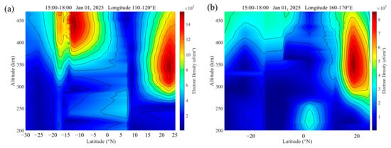
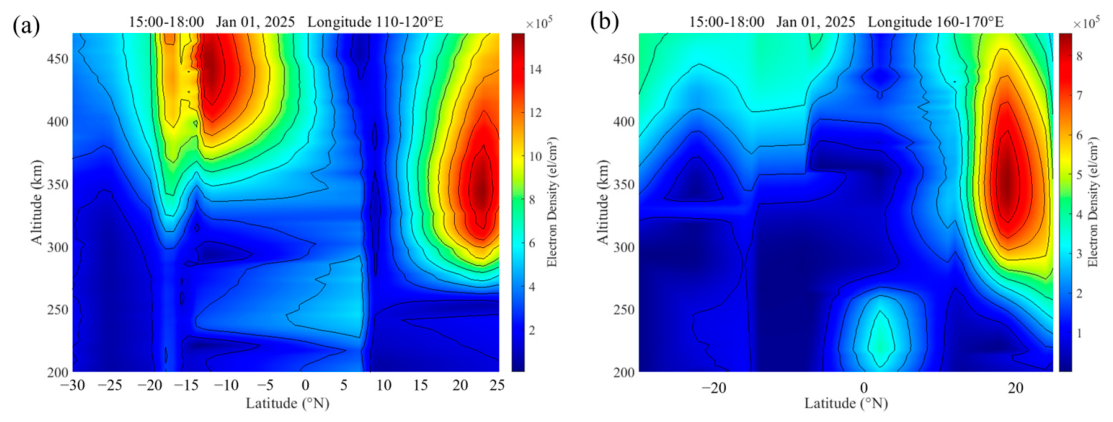
To explain the hemispheric asymmetry in the ionospheric storm response, we analyzed the latitude altitude Ne profiles around two ionospheric stations, Learmonth and Wake Island, from 15:00 to 18:00 UT. As shown in Figure 16a, a sharp and intense peak appears at an altitude of approximately 450 km at the Learmonth station site, indicating significant uplift of the ionosphere due to the transient penetrating electric field (PPEF) modulation. At lower altitudes (250–350 km), however, large areas are present where the equatorial ionization anomaly (EIA) characteristic of the low-latitude region has completely disappeared, revealing severe erosion of the ionosphere. Figure 16b for Wake Island shows a weaker peak, but the lower ionosphere (250–350 km) remains a continuous structure without obvious low-density regions. This stark contrast is caused by the two different physical processes.

Figure 16. Changes in latitude Ne profiles over (a) Learmonth region and (b) Wake Island 15:00–18:00 UT on 1 January.

First, the eastward PPEF during the storm caused a significant uplift of ionosphere over the Learmonth station, producing the high-altitude Ne peaks. Over the Wake Island longitude, however, weaker uplift occurred. Then, storm-enhanced circulation patterns, driven by enhanced geomagnetic fields, led to large spatial fluctuations in [O/N₂] ratio across different latitudes. January is summer in the Southern Hemisphere, and strong storm-induced and solar-driven circulations both flow towards the equator, transporting gases with a low O/N2 ratio from the auroral zone to low-latitude regions. This O/N₂ air mass directly affects the Learmonth station. In contrast, Wake Island, located in the Northern Hemisphere winter, experiences neither significant uplift nor transport of low-O/N₂ ratio air masses from the Arctic due to the influence of the polar background winds. Therefore, its Total Electron Content (TEC) remains slightly changed. At Learmonth, the combination of ionosphere uplift and low O/N₂ led to a net TEC decrease; at Wake Island, the absence of both processes resulted in no significant change.

5. Conclusions

Due to the intense solar activity, a large amount of energy is dispersed into space. When this energy enters the Earth, it affects the atmospheric–ionospheric system and causes geomagnetic storms. During geomagnetic storms, particle precipitation and electromagnetic energy injection into the upper atmosphere can cause an increase in neutral component density in the upper atmosphere. This leads to an increase in the ionization degree of the Earth’s ionosphere, making the distribution of ionospheric free electrons more non-uniform, resulting in ionospheric scintillation and ionospheric delay.

Since the end of December, the intense solar activity has led to a super geomagnetic storm on Earth on 1 January. The distribution of TEC and the degree of ionospheric disturbance show significant regional differences. The ionospheric disturbance in the Learmonth region of Australia is intense, with significant fluctuations in parameters, while the ionosphere in Wake Island in the Pacific is less affected. In the Learmonth region of Australia in the Southern Hemisphere, data analysis from ionosonde stations shows a significant decrease in f_oF₂, M3000F₂, and TEC in Australia, while h_mF₂ has increased.

In the classic middle latitude mechanism, summer equatorward circulation produces negative phases of ionospheric storms, while winter opposing circulation produces positive phases of ionospheric storms. However, this mechanism cannot be directly applied to low-latitude sites (~20°) in both hemispheres. Nevertheless, the seasonal asymmetry of thermospheric background conditions remains crucial; it explains why Learmonth exhibits a significant negative-phase storm while Wake Island shows little change. During the storm (1 January), the Southern Hemisphere was in summer while the Northern Hemisphere was in winter, leading to distinctly different large-scale circulation patterns. In the summer hemisphere, both storm-enhanced and solar-driven circulations produce strong equatorward winds. These winds transport air with a reduced O/N₂ ratio from the auroral zone to lower latitudes. The [O/N₂] ratio at Learmonth dropped sharply from about 0.6 to 0.25 during the storm-time. This low-O/N₂ air significantly enhanced electron recombination at lower altitudes (250–350 km), leading to decreased Ne in the lower part of the ionosphere. What is more, the equatorial ionization anomaly (EIA) pattern disappeared. In contrast, the [O/N₂] ratio at Wake Island remained above 0.7. The winter hemisphere is characterized by poleward background winds, which prevented the transport of low-O/N₂ air masses to Wake Island.

The PPEF further modulated this response; it caused strong ionospheric uplift over both longitudes, producing a high-altitude (450 km) Ne peak at Learmonth. However, this positive effect was disrupted due to the low-O/N₂ air, resulting in a net TEC decrease. At Wake Island, the PPEF uplift was much weaker, and no low-O/N₂ air reached the station because of the winter poleward winds. Consequently, the TEC stayed stable. These observations suggest that the net TEC change during storms at low latitudes depends not only on the presence of uplift, but on the balance between uplift and Ne loss. This work provides a new perspective for understanding low-latitude hemispheric differences during geomagnetic storms and highlights the importance of combining seasonal asymmetry, storm-induced composition changes, and PPEF modulation.

References

- Siscoe, G.; Schwenn, R. CME Disturbance Forecasting. Space Sci. Rev. 2006, 123, 453–470. [Google Scholar] [CrossRef]
- Singh, A.K.; Siingh, D.; Singh, R.P. Space Weather: Physics, Effects and Predictability. Surv. Geophys. 2010, 31, 581–638. [Google Scholar] [CrossRef]
- Harvey, K.L. The explosive phase of solar flares. Sol. Phys. 1971, 16, 423–430. [Google Scholar] [CrossRef]
- Veronig, A.; Temmer, M.; Hanslmeier, A.; Otruba, W.; Messerotti, M. Temporal aspects and frequency distributions of solar soft X-ray flares. Astron. Astrophys. 2012, 382, 1070–1080. [Google Scholar] [CrossRef]
- Eren, S.; Kilcik, A.; Atay, T.; Miteva, R.; Yurchyshyn, V.; Rozelot, J.P.; Ozguc, A. Flare-production potential associated with different sunspot groups. MNRAS 2017, 465, 68–75. [Google Scholar] [CrossRef]
- Winter, L.M.; Balasubramaniam, K. Using the maximum X-ray flux ratio and X-ray background to predict solar flare class. Space Weather 2015, 13, 286–297. [Google Scholar] [CrossRef]
- Browning, P.K.; Gordovskyy, M.; Schiavo, L.A.C.A.; Stewart, J. From Kink Instability to Magnetic Reconnection to Oscillations in Solar Flares. Fundam. Plasma Phys. 2024, 10, 100049. [Google Scholar] [CrossRef]
- Gonzalez, W.D.; Gonzalez, A.L.C.; Tsurutani, B.T. Dual-peak solar cycle distribution of intense geomagnetic storms. Planet. Space Sci. 1990, 38, 181–187. [Google Scholar] [CrossRef]
- Willis, D.M. The sudden commencement and first phase of a geomagnetic storm. J. Atmos. Terr. Phys. 1964, 26, 581–602. [Google Scholar] [CrossRef]
- Zolotukhina, N.; Polekh, N.; Kurkin, V.; Rogov, D.; Romanova, E.; Chelpanov, M. Ionospheric effects of St. Patrick’s storm over Asian Russia: 17–19 March 2015. J. Geophys. Res. Space Phys. 2017, 122, 2484–2504. [Google Scholar] [CrossRef]
- Buonsanto, M.J. Ionospheric storms—A review. Space Sci. Rev. 1999, 88, 563–601. [Google Scholar] [CrossRef]
- Boteler, D.H.; Pirjola, R.J.; Nevanlinna, H. The effects of geomagnetic disturbances on electrical systems at the earth’s surface. Adv. Space Res. 1998, 22, 17–27. [Google Scholar] [CrossRef]
- Li, L.; Jin, S. Ionospheric behaviors and characteristics in asian sector during the april 2023 geomagnetic storm with multi-instruments observations. J. Atmos. Sol.-Terr. Phys. 2024, 259, 106238. [Google Scholar] [CrossRef]
- De Jesus, R.; Sahai, Y.; Fagundes, P.R.; De Abreu, A.J.; Brunini, C.; Gende, M.; Bittencourt, J.A.; Abalde, J.R.; Pillat, V.G. Response of equatorial, low- and mid- latitude F-region in the american sector during the intense geomagnetic storm on 24–25 october 2011. Adv. Space Res. 2013, 1, 147–157. [Google Scholar] [CrossRef]
- De Abreu, A.J.; Correia, E.; De Jesus, R.; Venkatesh, K.; Macho, E.P.; Roberto, M.; Fagundes, P.R.; Gende, M. Statistical analysis on the ionospheric response over South American mid-and near high-latitudes during 70 intense geomagnetic storms occurred in the period of two decades. J. Atmos. Sol.-Terr. Phys. 2023, 245, 106060. [Google Scholar] [CrossRef]
- Fagundes, P.R.; Tsali-Brown, V.Y.; Pillat, V.G.; Arcanjo, M.O.; Venkatesh, K.; Habarulema, J.B.; Bolzan, M.J.A.; de Jesus, R.; De Abreu, A.J.; Tardelli, A.; et al. Ionospheric storm due to solar Coronal mass ejection in September 2017 over the Brazilian and African longitudes. Adv. Space Res. 2023, 71, 46–66. [Google Scholar] [CrossRef]
- Klimenko, M.V.; Klimenko, V.V.; Ratovsky, K.G.; Goncharenko, L.P.; Sahai, Y.; Fagundes, P.R.; De Jesus, R.; De Abreu, A.J.; Vesnin, A.M. Numerical modeling of ionospheric effects in the middle-and low-latitude F region during geomagnetic storm sequence of 9–14 September 2005. Radio Sci. 2011, 46, RS0D03. [Google Scholar] [CrossRef]
- Sahai, Y.; Becker-Guedes, F.; Fagundes, P.R.; Lima, W.L.C.; De Abreu, A.J.; Guarnieri, F.L.; Candido, C.M.N.; Pillat, V.G. Unusual ionospheric effects observed during the intense 28 October 2003 solar flare in the Brazilian sector. Ann. Geophys. 2007, 25, 2497–2502. [Google Scholar] [CrossRef]
- Venkatesh, K.; Tulasi Ram, S.; Fagundes, P.R.; Seemala, G.K.; Batista, I.S. Electrodynamic disturbances in the brazilian equatorial and low-latitude ionosphere on st. patrick’s day storm of 17 march 2015. J. Geophys. Res. Space Phys. 2017, 122, 4553–4570. [Google Scholar] [CrossRef]
- Chernogor, L.F.; Rozumenko, V.T. Earth–atmosphere–geospace as an open nonlinear dynamical system. Radio Phys. Radio Astron. 2008, 13, 120–137. Available online: https://api.semanticscholar.org/CorpusID:130788183 (accessed on 20 May 2025).
- Chernogor, L.F. The earth–atmosphere–geospace system: Main properties and processes. Int. J. Remote Sens. 2011, 32, 3199–3218. [Google Scholar] [CrossRef]
- Skone, S.; Yousuf, R. Performance of satellite-based navigation for marine users during ionospheric disturbances. Space Weather 2016, 5, S01006. [Google Scholar] [CrossRef]
- Astafyeva, E.; Yasyukevich, Y.; Maksikov, A.; Zhivetiev, I. Geomagnetic storms, super-storms, and their impacts on gps-based navigation systems. Space Weather 2016, 12, 508–525. [Google Scholar] [CrossRef]
- Coster, A.J.; Colerico, M.J.; Foster, J.C.; Rideout, W.; Rich, F. Longitude Sector Comparisons of Storm Enhanced Density. Geophys. Res. Lett. 2007, 34, 2007GL030682. [Google Scholar] [CrossRef]
- Kuai, J.; Ma, Q.; Yu, T.; Wu, K.; Sun, H.; Zhang, Y. Significant East-West Electron Density Differences Occurring in Less than 30° Longitude over the Ocean during the Recovery Phase of a Strong Geomagnetic Storm in Solar Minimum. J. Geophys. Res. Space Phys. 2025, 130, e2024JA033549. [Google Scholar] [CrossRef]
- Mendillo, M.; He, X.-Q.; Rishbeth, H. How the Effects of Winds and Electric Fields in F2-Layer Storms Vary with Latitude and Longitude: A Theoretical Study. Planet. Space Sci. 1992, 40, 595–606. [Google Scholar] [CrossRef]
- Yizengaw, E.; Groves, K.M. Longitudinal and Seasonal Variability of Equatorial Ionospheric Irregularities and Electrodynamics. Space Weather 2018, 16, 946–968. [Google Scholar] [CrossRef]
- Picanço, G.A.D.S.; Fagundes, P.R.; Moro, J.; Nogueira, P.A.B.; Muella, M.T.; Denardini, C.M.; Resende, L.C.A.; Silva, L.A.D.; Laranja, S.R. Dynamics of polar-equatorial ionospheric irregularities during the 10–13 october 2024 superstorm. ESS. Open Arch. 2024, preprint. [Google Scholar] [CrossRef]
- Nicolls, M.J.; Kelley, M.C.; Coster, A.J.; González, S.A.; Makela, J.J. Imaging the structure of a large-scale TID using ISR and TEC data. Geophys. Res. Lett. 2004, 31, L09812. [Google Scholar] [CrossRef]
- Ren, X.; Mei, D.; Liu, H.; Zhang, X. Investigation on horizontal and vertical traveling ionospheric disturbances propagation in global-scale using GNSS and multi-LEO satellites. Space Weather. 2022, 20, e2022SW003041. [Google Scholar] [CrossRef]
- Tang, J.; Gao, X.; Li, Y.; Zhong, Z. Study of ionospheric responses over China during September 7–8, 2017 using GPS, Beidou (GEO), and Swarm satellite observations. GPS Solut. 2022, 26, 55. [Google Scholar] [CrossRef]
- Jin, S.; Park, J.U.; Wang, J.L.; Choi, B.K.; Park, P.H. Electron density profiles derived from ground-based GPS observations. J. Navig. 2006, 59, 395–401. [Google Scholar] [CrossRef]
- Jin, S.; Park, J.U. GPS ionospheric tomography: A comparison with the iri-2001 model over south korea. Earth Plan. Space 2007, 59, 287–292. [Google Scholar] [CrossRef]
- Heise, S.; Jakowski, N.; Wehrenpfennig, A.; Reigber, C.; Lühr, H. Sounding of the topside ionosphere/plasmasphere based on GPS measurements from CHAMP: Initial results. Geophys. Res. Lett. 2002, 29, 44. [Google Scholar] [CrossRef]
- Liu, L.; Zou, S.; Yao, Y.; Aa, E. Multi-scale ionosphere responses to the May 2017 magnetic storm over the Asian sector. GPS Solut. 2020, 24, 26. [Google Scholar] [CrossRef]
- Jin, S.; Wang, Q.; Dardanelli, G. A review on multi-GNSS for earth observation and emerging applications. Remote Sens. 2022, 14, 3930. [Google Scholar] [CrossRef]
- Heki, K.; Enomoto, Y. Mw dependence of the preseismic ionospheric electron enhancements. J. Geophys. Res. Space Physics. 2015, 120, 7006–7020. [Google Scholar] [CrossRef]
- Shinbori, A.; Otsuka, Y.; Sori, T.; Nishioka, M.; Perwitasari, S.; Tsuda, T.; Nishitani, N. Electromagnetic conjugacy of ionospheric disturbances after the 2022 Hunga Tonga-Hunga Ha’apai volcanic eruption as seen in GNSS-TEC and SuperDARN Hokkaido pair of radars observations. Earth Plan. Space 2022, 74, 106. [Google Scholar] [CrossRef]
- Alizadeh, M.M.; Schuh, H.; Todorova, S.; Schmidt, M. Global ionosphere maps of VTEC from GNSS, satellite altimetry, and Formosat-3/COSMIC data. J. Geod. 2011, 85, 975–987. [Google Scholar] [CrossRef]
- Kotulak, K.; Zakharenkova, I.; Krankowski, A.; Cherniak, I.; Wang, N.; Fron, A. Climatology characteristics of ionospheric irregularities described with GNSS ROTI. Remote Sens. 2020, 12, 2634. [Google Scholar] [CrossRef]
- Demelash, S.; Kassa, T. Ionospheric irregularities observed during the geomagnetic storm of March 2015 and June 2015 over Ethiopia. Adv. Space Res. 2023, 72, 1290–1303. [Google Scholar] [CrossRef]
- Seemala, G.K.; Valladares, C.E. Statistics of total electron content depletions observed over the South American continent for the year 2008. Radio Sci. 2011, 46, RS5019. [Google Scholar] [CrossRef]
- Wu, F.; Yao, D.; Yu, C. An investigation into the influence of solar flares and geomagnetic storms on the f2 layer of the ionosphere in western europe during march 2024. Adv. Space Res. 2025, 75, 936–952. [Google Scholar] [CrossRef]
- Balan, N.; Shiokawa, K.; Otsuka, Y.; Kikuchi, T.; Vijaya Lekshmi, D.; Kawamura, S.; Yamamoto, M.; Bailey, G.J. A Physical Mechanism of Positive Ionospheric Storms at Low Latitudes and Midlatitudes. J. Geophys. Res. 2010, 115, A02304. [Google Scholar] [CrossRef]
Disclaimer/Publisher’s Note: The statements, opinions and data contained in all publications are solely those of the individual author(s) and contributor(s) and not of MDPI and/or the editor(s). MDPI and/or the editor(s) disclaim responsibility for any injury to people or property resulting from any ideas, methods, instructions or products referred to in the content. |
© 2026 by the authors. Licensee MDPI, Basel, Switzerland. This article is an open access article distributed under the terms and conditions of the Creative Commons Attribution (CC BY) license.