PM_2.5 Prediction Based on LSTM Weighted by K-Nearest Neighbor Algorithm

Abstract

Accurate prediction of PM_2.5 concentration is essential for public health and environmental protection, and specifically crucial for the management of the availability of sufficient health personnel during adverse health episodes. However, its nonlinearity, variability, and complexity make this task challenging. This study proposes a long short-term memory (LSTM) weighted by K-nearest neighbor (KNN) algorithm (namely Weighted KNN-LSTM Model) that can effectively predict the PM_2.5 concentration time series. Firstly, the K-nearest neighbors of each time point are sought based on the Euclidean distance within the data time range. Given that neighboring observations typically exert a more pronounced influence than distant ones in spatial processes, weights are accordingly assigned to these neighbors to quantitatively reflect their relative importance in the analysis. Subsequently, after the initial data is processed by the weighted KNN algorithm, it is reorganized and transformed into a reconstructed dataset with a size K times that of the original data. The data used for model training and the data used for evaluating the model’s prediction performance are completely independent, and the test dataset is never involved in the model training process to ensure the authenticity and reliability of the prediction performance evaluation. Then, the LSTM neural network model is trained on this new dataset to enhance its generalization ability. The experimental results show that the weighted KNN-LSTM model exhibits excellent predictive performance in predicting PM_2.5 concentration. It is important to note that the dataset used to evaluate the model’s performance was strictly independent from the data used to train the model. This separation ensures that the reported accuracy reflects true predictive capability rather than mere fitting quality. The model provides a technical reference for hourly PM_2.5 concentration prediction in Nanchang City, and the prediction results can be used as an auxiliary reference for regional air quality monitoring; the application of the model in heavy pollution warnings needs to be further optimized and verified by combining multi-source data such as meteorology, which provide reliable data support for the formulation of dynamic emission reduction policies.

1. Introduction

The frequent occurrence of haze events has become a serious environmental problem in China and even globally, and PM_2.5 is the main contributor to haze weather. The increase in its concentration not only affects human health, but also causes climate change [1,2,3]. The formation of PM_2.5 (fine particulate matter) is a complex physical and chemical process, involving both primary emissions and secondary generation [4]. Primary emissions refer to the direct release of particulate matter by pollution sources, including industrial production processes, vehicle exhaust emissions, dust emissions, and various human activities [5]. Secondary generation is the most important source of PM_2.5, especially during severe pollution periods. It refers to the transformation of gaseous precursors, including sulfur dioxide (SO₂), nitrogen oxides (NO_x), ammonia (NH₃), and volatile organic compounds (VOCs), into solid or liquid particulate matter through a series of physical and chemical processes in the atmosphere [6,7].

In China, PM_2.5 pollution is particularly serious and has become one of the main pollutants. According to statistics, out of 339 prefecture-level and above cities in China, as many as 86 cities have PM_2.5 concentrations that exceed the national standard for consecutive time series, which means that nearly a quarter of urban residents are living in environments with PM_2.5 concentration time series exceeding the standard [8,9]. Therefore, exploring effective PM_2.5 concentration prediction models is crucial for human health and environmental protection. Accurate predictions enable health authorities to anticipate spikes in respiratory illnesses, thereby optimizing the deployment and availability of medical staff during severe pollution episodes.

At present, in order to address the pollution problem of PM_2.5, many researchers are seeking better prediction methods to analyze the PM_2.5 concentration time series with the aim of formulating effective planning and response measures. There are many employed time series forecasting methods such as linear regression [10], the autoregressive integrated moving average (ARIMA) model [11,12] and the BP neural network [13,14], among others. For example, three statistical models based on autoregression (AR), moving average (MA) and ARIMA models were applied to the datasets of PM_2.5 concentrations of Delhi and Bengaluru, to conduct 1-day-ahead and 7-day-ahead forecasting [15]. But the above study also pointed out that other topographical and meteorological parameters need to be incorporated to develop better models and to account for the impacts of these parameters in the research. This is because the PM_2.5 concentration is jointly affected by meteorological factors such as temperature and wind speed, as well as other atmospheric pollutants such as O₃, CO and SO₂ [3,15]. In fact, PM_2.5 concentration is also significantly influenced by other key weather conditions including precipitation, relative humidity, and atmospheric pressure. These meteorological factors regulate the diffusion, deposition, and chemical transformation of PM_2.5, thereby exerting a crucial impact on its concentration levels. For instance, high relative humidity can promote the hygroscopic growth of PM_2.5 particles, leading to an increase in their concentration; strong winds facilitate the diffusion of pollutants, reducing local PM_2.5 levels, and precipitation can scavenge particulate matter from the atmosphere, resulting in a temporary decrease in concentration. Meteorological factors are the core driving factors affecting the spatial and temporal distribution of PM_2.5 concentration, and the integration of meteorological data is an essential link for improving the physical interpretability and prediction upper limit of PM_2.5 prediction models. In the field of atmospheric environmental science research in 2025, the construction of PM_2.5 prediction models based on pollutant concentration data alone has obvious limitations, and the combination of multi-source data such as meteorology and anthropogenic activities has become a mainstream research direction. Therefore, in order to more accurately predict PM_2.5 concentration, researchers often chose a multiple linear regression method to make predictions by comprehensively analyzing multiple variables. This type of model mainly relies on the intrinsic correlation changes in sequence data for analysis, and has low efficiency in processing large-scale data. More importantly, these methods often yield large calculation errors and have slow calculation speeds, which undoubtedly increases the uncertainty of predictions. Nowadays, with the rapid development and continuous improvement in artificial intelligence (AI) technology, AI exhibits higher efficiency and accuracy in processing big data, which can more effectively explore the potential patterns and trends of data, thus providing more reliable and accurate predictions. As a result, more and more scholars are actively exploring AI models to predict PM_2.5 concentration.

To improve the accuracy of AI and atmospheric diffusion models, many scholars have combined conventional air quality models with machine learning or AI models to forecast PM_2.5 concentration [16,17]. They do so to suggest combined and synoptic variables, in addition to conventional surface meteorological and air quality variables for developing AI-based high PM event prediction models [1]. However, traditional AI models also suffer from low accuracy in predicting PM_2.5 concentration. This is because such models have some drawbacks, such as cumbersome feature engineering, weak generalization ability, and limited ability to handle nonlinear problems, whereas deep learning (DL) could effectively handle these problems. With the development of DL algorithms, time series models can play a huge role in time-dependent PM_2.5 concentration forecasting [16,18]. These models can identify nonlinear relationships between input and output variables by constructing multi-layer neural networks, effectively extracting historical information features from data, and accurately capturing the key factors that affect PM_2.5 concentration, thus enabling more accurate PM_2.5 concentration prediction. Crucially, time series data of PM_2.5 possess a “memory” of past situations; this temporal dependency allows models to deduce future expectations of air quality based on historical trends and patterns. For instance, Pathak et al. [19] proposed a novel attention-based deep learning framework. By leveraging the attention mechanism, this framework enables the exploration of long-term temporal dependencies in the vector space. Combined with the inherent capability of the hybrid deep learning (DL) model, which integrates convolutional neural networks (CNNs) and long short-term memory (LSTM) to capture short-term temporal dependencies within the feature space, this framework achieves accurate prediction of PM_2.5 pollutant levels. Additionally, based on the spatial interaction hypothesis, Shi et al. developed a balanced social long short-term memory (BS-LSTM) neural network, which has also been successfully applied to PM_2.5 concentration prediction [20].

Our research team has previously proposed a prediction model (namely EEMD-ALSTM) based on Ensemble Empirical Mode Decomposition (EEMD), attention mechanism and LSTM for PM_2.5 concentration prediction, and the prediction results showed that the EEMD-ALSTM model had superior predictive performance [21]. Moreover, we have further developed DL models that integrate multiple algorithms to predict PM_2.5 concentration, such as LASSA-LGB that is integrated with Sparrow Search Algorithm (SSA) and optimized Light Gradient Boosting Machine (LightGBM) [22], the mWOA-SVR model based on Support Vector Regression (SVR) and modified Whale Optimization Algorithm (WOA) [23], the PSO- CPU-GPU-SVR model based on the Particle Swarm Optimization (PSO), Central Processing Unit (CPU), Graphics Processing Unit (GPU) and SVR [24], and a stacking fusion algorithm fused by the eXtreme Gradient Boosting (XGBoost), LightGBM and Random Forest (RF) [25].

Why are we exploring so many PM_2.5 concentration prediction methods? This is because there are several main research gaps as follows. (1) Deficiencies in existing combination methods—although many methods and models have been proposed to predict PM_2.5, there is still a gap in the use of comprehensive methods for prediction. Today’s research usually uses a single model, but lacks research that combines traditional statistical methods, physics-based models and machine learning methods, thus resulting in a lack of comprehensiveness in prediction results. (2) Neglect of the regional characteristics of PM_2.5 pollution—the meteorological and air pollution characteristics of various regions are different, which leads to varying adaptability of different model methods in predicting air pollution in different regions. It is possible that a certain method may have good predictive performance in one region but poor predictive performance in another region. Current research often overlooks such regional differences and lacks targeted prediction methods for specific areas. Notably, the geographical location, climate conditions (e.g., monsoon patterns, temperature ranges), and pollutant emission sources (e.g., industrial structure, energy consumption types) vary significantly across different cities. For example, northern Chinese cities are more affected by coal combustion for heating in winter, while southern cities may face greater pressure from vehicle exhaust and industrial emissions. These differences result in distinct PM_2.5 generation and diffusion mechanisms, making it difficult for a single model trained on data from one city to achieve consistent prediction accuracy in other regions. Therefore, the lack of cross-regional validation greatly limits the generalizability of existing models. (3) Inadequate handling of uncertainties in the prediction process—there are various uncertainties in the process of predicting air pollution concentration, including observation errors, model parameter uncertainties and meteorological condition uncertainties. The lack of research on uncertain factors in current forecasting can be addressed by strengthening the study of uncertain factors to enhance the reliability of prediction results.

Furthermore, the current models rarely consider anthropogenic activity indicators such as traffic flow, industrial emission intensity, energy consumption, and seasons/holidays. These factors are important drivers of PM_2.5 concentration changes. For example, peak traffic hours usually lead to an increase in vehicle exhaust emissions, resulting in a rise in PM_2.5 concentration; industrial production activities may have different emission intensities on working days and holidays; and seasonal changes (e.g., winter heating, summer high temperatures) can also affect the generation and accumulation of PM_2.5. Ignoring these anthropogenic factors limits the model’s ability to capture complex nonlinear relationships between PM_2.5 and its influencing factors.

In view of the complex hybrid models proposed by the research team in the early stage (such as EEMD-ALSTM, LASSA-LGB, mWOA-SVR, etc.), which have high model complexity and high requirements for computing resources and data quality, this study chooses to construct a lightweight Weighted KNN-LSTM model with a relatively simple architecture. The core research objective of this study is to explore the feasibility of improving the prediction accuracy of PM_2.5 concentration by introducing a weighted KNN-based data reconstruction strategy on the basis of the classic LSTM model, and to provide a lightweight and easy-to-implement technical solution for small and medium-sized cities with limited monitoring data and computing resources. Although the weighted KNN technology is a basic machine learning method, this study innovatively applies it to the data preprocessing stage of the LSTM model for PM_2.5 time series prediction, and verifies the effectiveness of the weighted mechanism in improving the model’s ability to capture the temporal correlation of PM_2.5 concentration through comparative experiments. The lightweight model design is more in line with the actual application needs of regional environmental monitoring departments with limited technical and resource conditions.

In this work, our research team aims to propose a new model for PM_2.5 prediction, namely the weighted KNN-LSTM model based on LSTM weighted by the KNN algorithm. Specifically, in accordance with the principle that the greater the distance, the smaller the importance, and the smaller the distance, the greater the importance, we assign corresponding weights to the nearest neighbors to reflect the relative importance of different neighbors, and then seek the KNN of each time point based on the Euclidean distance within the data time range. Then, after the initial data is processed by the weighted KNN algorithm, it is reorganized and transformed into a reconstructed dataset with a size K times that of the original data. Next, the LSTM neural network model is trained on this new dataset to enhance its generalization ability and achieve accurate prediction of PM_2.5 concentrations. PM_2.5 concentration time series have inherent memory of historical air quality conditions, and the temporal dependence contained in the sequence can be used to deduce the future expectation of air quality, which is the theoretical basis for using time series models to predict PM_2.5 concentration. The experimental results show that the weighted KNN-LSTM model exhibits excellent predictive performance in predicting PM_2.5 concentration, which achieves higher prediction accuracy than other comparative models. However, it should be emphasized that the model’s performance in other regions remains untested, and its ability to capture extreme PM_2.5 concentration outliers and sudden heavy pollution events has not been specifically evaluated. Therefore, the claim that the model can support “heavy pollution early warning” requires further empirical verification.

This study’s conclusions contribute to the accurate prediction of air quality in Nanchang, thereby it provides a scientific basis for formulating targeted strategies to improve regional air quality and alleviating the adverse impacts of air pollution on public health.

2. Data and Methods

2.1. Data Source

The experimental study data chosen in this work include PM_2.5 and five related air pollution concentration indicators, spanning from 0:00 on 1 February 2017 to 19:00 on 22 December 2018 in Nanchang City. The time interval between adjacent time points is 1 h. There are a total of 6 characteristic columns in the data, including PM_2.5, PM₁₀, SO₂, CO, NO₂ and O₃. The dataset of Nanchang City consists of 15,565 samples, with 80% used as the training set and 20% used as the testing set. We explicitly emphasize that the data used to evaluate the model’s performance (the 20% testing set) were not used in any stage of model training or parameter tuning. It is necessary to state this clearly so that young scientists learn that they cannot use the same data for model development and evaluation, as doing so would just assess the quality of fit, but provide no information about the quality of the prediction. This study uses the 2017–2018 Nanchang City air pollutant concentration data as the research basis for the preliminary verification of the Weighted KNN-LSTM model framework; in the follow-up research, the research team will supplement the latest PM_2.5 concentration monitoring data of Nanchang City from 2019 to 2024, and integrate multi-source data such as meteorology and anthropogenic activities for model optimization and re-verification to improve the timeliness and applicability of the research results.

Moreover, due to objective data availability limitations, it should be noted that this study did not include meteorological data (e.g., wind speed, precipitation, relative humidity, atmospheric pressure) and anthropogenic activity indicators (e.g., traffic flow, industrial emission intensity, energy consumption, seasons/holidays) due to data availability limitations. These factors are known to have significant and direct impacts on PM_2.5 concentration generation, diffusion and transformation, and their exclusion is a key limitation of this study, which may affect the model’s ability to capture the complete and complex nonlinear changes in PM_2.5 concentration. The lack of meteorological data is the main limitation of this study. Meteorological factors such as wind speed, temperature inversion, and precipitation are the key reasons for the sudden change in PM_2.5 concentration. The absence of such data makes the model unable to explain the physical mechanism of PM_2.5 concentration change, and it only can capture the numerical correlation between pollutant concentrations, resulting in the insufficient interpretability of the model’s prediction results.

2.2. KNN Algorithm

The KNN (K-nearest neighbor) algorithm, also known as the KNN algorithm, is a machine learning technique commonly used in classification and regression [26]. It is still widely used today. Due to its significant advantages in processing multidimensional and even high-dimensional data, KNN is widely used in various fields such as data mining [27,28] and pattern recognition [29]. The basic principle of KNN algorithm in classification is to use a pre-set distance formula to calculate the distance between unknown class samples and known class samples [30]. By calculating the distance, the nearest K samples are found, and the category of the unknown class sample is determined based on the majority category of the K samples. A significant advantage of this algorithm is that it does not require pre-training of the model and can be directly processed based on the dataset, thus having high adaptability to new data. In addition, the KNN algorithm is also applied in regression problems, which infers the predicted value of the test sample based on the actual values of the neighboring samples.

2.3. LSTM Neural Network

(1)

Recurrent Neural Network (RNN)

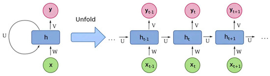
Recurrent neural network (RNN) is a type of neural network specifically designed for processing sequence data [31]. Compared to traditional neural networks, it pioneered the “memory” mechanism, allowing it to learn the correlations between consecutive samples and retain historical data information when processing current data. Therefore, RNN has a strong ability to learn and predict sequential data [31,32]. For example, in tasks such as natural language processing and speech recognition, traditional feedforward neural networks cannot effectively capture dependencies in sequences. However, RNN solves this problem by introducing cyclic connections, allowing the network to store and utilize past information. Therefore, in natural language processing, RNN is widely used in tasks such as machine translation, text generation, and sentiment analysis. In the field of speech recognition, RNN can effectively process continuous speech signals and achieve high-precision speech recognition. In addition, the role of RNN cannot be ignored in fields such as time series prediction and stock market analysis. The theoretical model is shown in Figure 1.

Figure 1. RNN structure.

Based on the RNN structure diagram, in order to better explain the principle of the RNN model, the formulas involved are as follows:

$$h_t=F(W{x}_t+U{h}_{t-1})$$

(1)

$$y_t=G(V{h}_t)$$

(2)

The input is x, the output is y, the intermediate state of the hidden layer is h, and the weights U, W and V in the network are equal at every moment. F(·) and G(·) are activation functions.

The above formula indicates the calculation process of a recurrent neural network unit. Based on its calculation process, it can be concluded that the output at the current time is not only related to the input at the current time, but also to the hidden state of the previous neural unit. Thus, it can be concluded that RNN has memory function, but the RNN is not perfect. As the depth of the network increases, it cannot retain historical data from a long time ago, such that the point where the output of the current time distribution is only related to the historical data from adjacent steps. Furthermore, in the backpropagation process, it is easy to encounter problems such as vanishing or exploding gradients, making it difficult to train the model.

(2)

Long Short-Term Memory Network

Therefore, RNN has a strong ability to learn and predict sequential data. The inherent memory mechanism of these models means that the current state of PM_2.5 concentration is not isolated but is deeply influenced by previous time steps. Consequently, the time series of PM_2.5 data have memory of the past situation and hence can be used to deduce future expectation of air quality. Long short-term memory (LSTM) is an improved form of RNN, which is commonly used for processing long time series and is widely used in fields such as natural language processing, speech recognition and image processing [33].

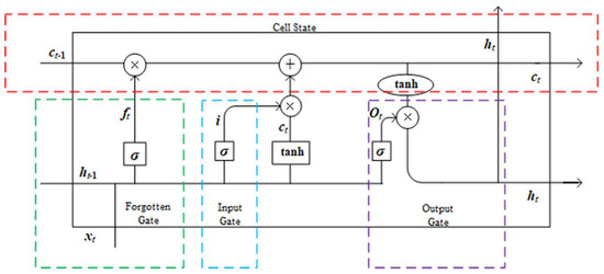
The design of the LSTM model is to address some of the drawbacks of RNN; for instance, RNN receives all input information indiscriminately with an unfocused memory mechanism, memorizing both the key data that should be retained and the redundant data that should be discarded [34,35]; in addition, when the time series is too long, the new information in the RNN will overwrite the old information, leading to the loss of long-term memory information. Therefore, the performance of the RNN model is not good when processing long time series. For this purpose, LSTM introduces a cell state and a set of gating mechanisms to achieve precise control over data transmission and retention [36]. The design of this cell control mechanism in LSTM means that when calculating the output at the current time, the model not only considers the output of the previous time step and the input of the current time step, but also uses the previous cell state to store important historical information. After processing the data at the current time, each node unit in LSTM not only outputs a result at the current time, but also transmits the current node unit state (also known as the hidden state) to the next LSTM unit. Due to its cell control mechanism and the continuous transmission of node unit states, LSTM can effectively process historical information with very long time intervals, solving the problem of the poor performance of RNN in processing long sequence data. This makes the LSTM model significantly advantageous in analyzing sequence data with long-term dependencies. The LSTM neural network structure is shown in Figure 2.

Figure 2. Schematic of LSTM structure [21].

2.4. Principle of Weighted KNN-LSTM Model

To some extent, each learning model has some limitations and cannot fully adapt to all types of data, nor can its prediction accuracy reach 100%. In order to further improve the accuracy of prediction, it is possible to consider combining multiple models to fully utilize the advantages of each model, and select the optimal integrated model for practical application. This method is also known as an ensemble learning algorithm. Ensemble learning algorithms can be classified into Bagging, Boosting and Stacking ensemble learning methods based on their structural characteristics. While the Bagging and Boosting algorithms use the principles of voting and weighted averaging, respectively, the Stacking algorithm takes a different approach by constructing a new model to retrain the predictions of multiple learners. The basic idea is to use multiple base learners to learn from the training data separately, and then use the outputs of these base learners as new features to input into the meta-learner for training. Finally, the meta-learner provides the prediction results.

In order to handle the temporal correlation influence between nodes in the time series, this study first uses the KNN algorithm to select K time points that have an impact on the current time point by using the Euclidean distance formula, and assigns corresponding weights to these K time points to represent the degree of influence of K-nearest neighbor time points on the current time point. Then, the feature data of the K neighboring time points are concatenated in series to construct reconstructed dataset with a size K times that of the original data. When determining weights, we follow a principle: the smaller the distance, the greater the weight and the higher the importance; The larger the distance, the smaller the weight, and the lower the importance. Therefore, this article chooses the reciprocal of distance as the weight. The distance between time nodes is calculated using Euclidean distance, which is defined as follows:

$$dist=\sqrt{{\displaystyle {\sum }_{m=1}^s(x_{i,m}-x_{j,m})}},\hspace{1em}i,j=1,2,\dots ,n$$

(3)

where x_i,_m and x_j,_m represent the mth feature value for time point i and j respectively; s is the number of features of each time point sample, and dist indicates the distance between the time point i and j.

After calculating the distance between time points based on the distance formula, the corresponding weights can be calculated using the obtained distance. The calculation formula is as follows:

$$w_{i,j}=\left\{\begin{array}{l}{\displaystyle \frac{1}{dist}}\begin{array}{cc},& i\ne j\end{array}\\ 1\begin{array}{cc},& i=j\end{array}\end{array}\right.$$

(4)

where w_i,j is the weight assigned to time point j as the nearest neighbor of time point i.

After obtaining the corresponding weights of the nearest neighbors, the calculated weights can be multiplied by the features at the corresponding time points to obtain data with weight effects. The formulas involved are as follows:

$${\mathit{x}}_i^{(k)}=\left[x_{i,1}^{(k)},x_{i,2}^{(k)},\dots ,x_{i,s}^{(k)}\right]$$

(5)

$$a_i^{(k)}{\mathit{x}}_i^{(k)}=\left[a_i^{(k)}{x}_{i,1}^{(k)},a_i^{(k)}{x}_{i,2}^{(k)},\dots ,a_i^{(k)}{x}_{i,s}^{(k)}\right]$$

(6)

where ${\mathit{x}}_i^{(k)}$ denotes the k-th nearest neighbor at time point i, $x_{i,s}^{(k)}$ represents the s feature of the k-th nearest neighbor at time point i, and $a_i^{(k)}$ is the weight of ${\mathit{x}}_i^{(k)}$.

Each time point sample has K-nearest neighbors, and the weighted data can be written in the form of column vectors, so that

$$S_1={\left[\begin{array}{c}{a}_1^{(1)}{x}_1^{(1)}\\ a_2^{(1)}{x}_2^{(1)}\\ ⋮\\ a_n^{(1)}{x}_n^{(1)}\end{array}\right]}_{n\times m},\hspace{1em}{S}_2={\left[\begin{array}{c}{a}_1^{(2)}{x}_1^{(2)}\\ a_2^{(2)}{x}_2^{(2)}\\ ⋮\\ a_n^{(2)}{x}_n^{(2)}\end{array}\right]}_{n\times m},\hspace{1em}\dots ,\hspace{1em}{S_k=\left[\begin{array}{c}{a}_1^{(k)}{x}_1^{(k)}\\ a_2^{(k)}{x}_2^{(k)}\\ ⋮\\ a_n^{(k)}{x}_n^{(k)}\end{array}\right]}_{n\times m}$$

(7)

where S₁, S₂ and S_k are the matrix composed of the first, second and K-th nearest neighbor feature data at each time point respectively.

Finally, K matrices S₁, S₂, …, S_k could be concatenated to obtain a new data matrix with a size K times that of the original data matrix, which can be expressed as

$$S^{\prime }={\left[S_1,S_2,\dots ,S_k\right]}_{n\times km}$$

(8)

To clearly display the content, it can be expanded as follows:

$$S^{\prime }={\left[\begin{array}{cccccccccc}{a}_1^{(1)}{x}_{1,1}^{(1)}& \dots & a_1^{(1)}{x}_{1,m}^{(1)}& a_1^{(2)}{x}_{1,1}^{(2)}& \dots & a_1^{(2)}{x}_{1,m}^{(2)}& \dots & a_1^{(k)}{x}_{1,1}^{(k)}& \dots & a_1^{(k)}{x}_{1,m}^{(k)}\\ a_2^{(1)}{x}_{2,1}^{(1)}& \dots & a_2^{(1)}{x}_{2,m}^{(1)}& a_2^{(2)}{x}_{2,1}^{(2)}& \dots & a_2^{(2)}{x}_{2,m}^{(2)}& \dots & a_2^{(k)}{x}_{2,1}^{(k)}& \dots & a_2^{(k)}{x}_{2,m}^{(k)}\\ ⋮& \dots & ⋮& ⋮& \dots & ⋮& \dots & ⋮& \dots & ⋮\\ a_n^{(1)}{x}_{n,1}^{(1)}& \dots & a_n^{(1)}{x}_{n,m}^{(1)}& a_n^{(2)}{x}_{n,1}^{(2)}& \dots & a_n^{(2)}{x}_{n,m}^{(2)}& \dots & a_n^{(k)}{x}_{n,1}^{(k)}& \dots & a_n^{(k)}{x}_{n,m}^{(k)}\end{array}\right]}_{n\times m}$$

(9)

where $S^{\prime }$ realizes K-fold data reconstruction, which contains the weighted feature data of all time points and their K-nearest neighbors. Each row and column of the matrix $S^{\prime }$ respectively represents the integrated weighted data of each feature and different time points with their K-nearest neighbors.

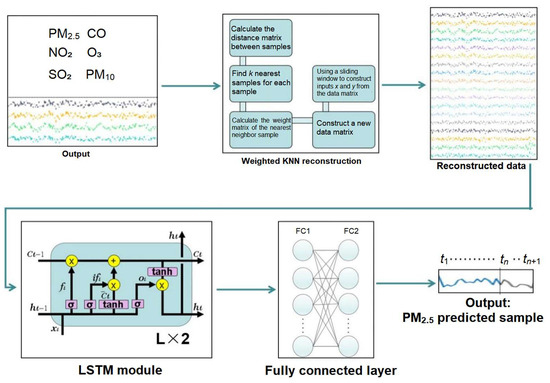
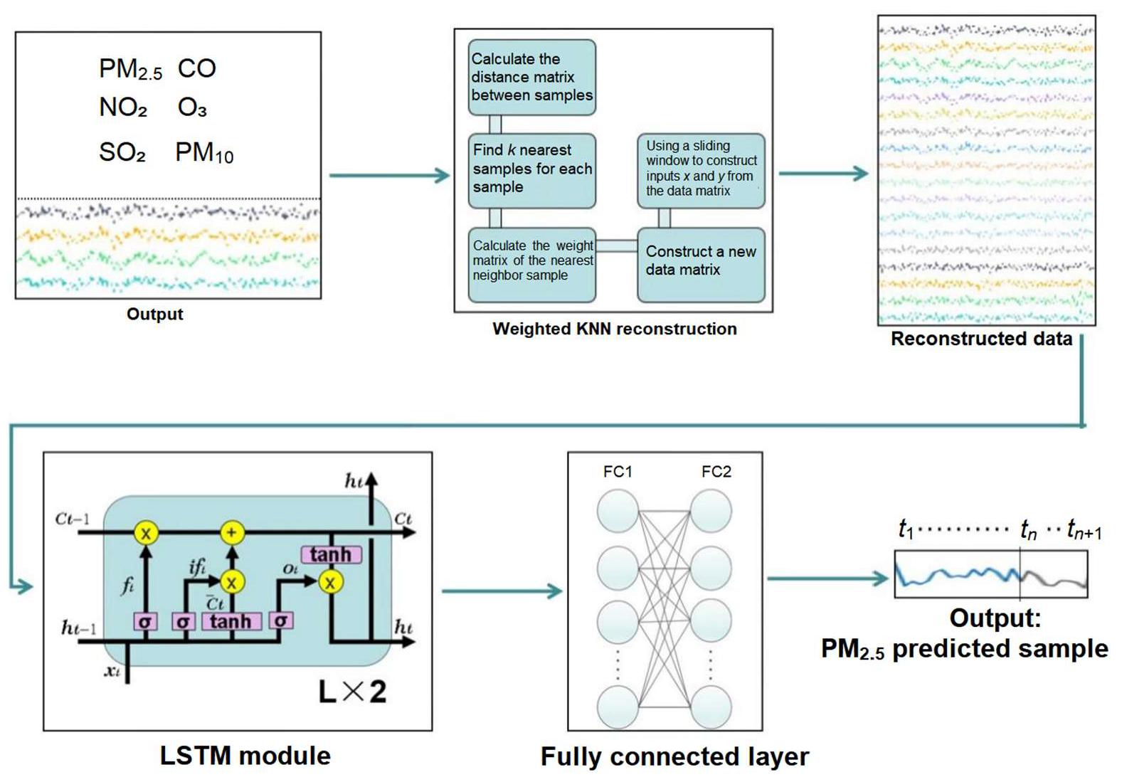
Subsequently, in combination with the LSTM model, the K-fold reconstructed data is used as the network input to predict PM_2.5 concentration. Due to its ability to capture long-term dependencies in time series, the LSTM model can more accurately predict future PM_2.5 concentrations. The structure of the entire weighted KNN-LSTM model is shown in Figure 3.

Figure 3. The structure of weighted KNN-LSTM model.

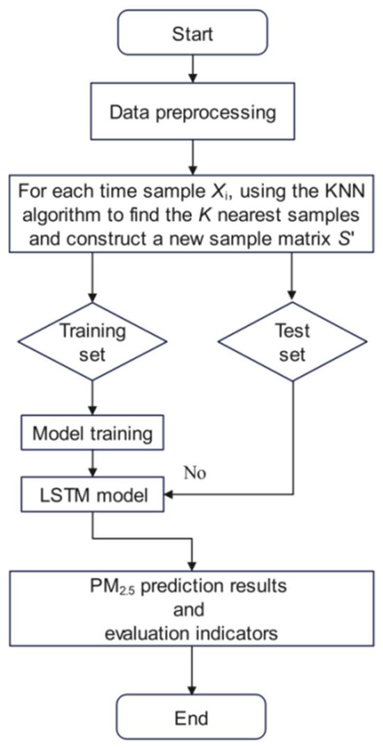
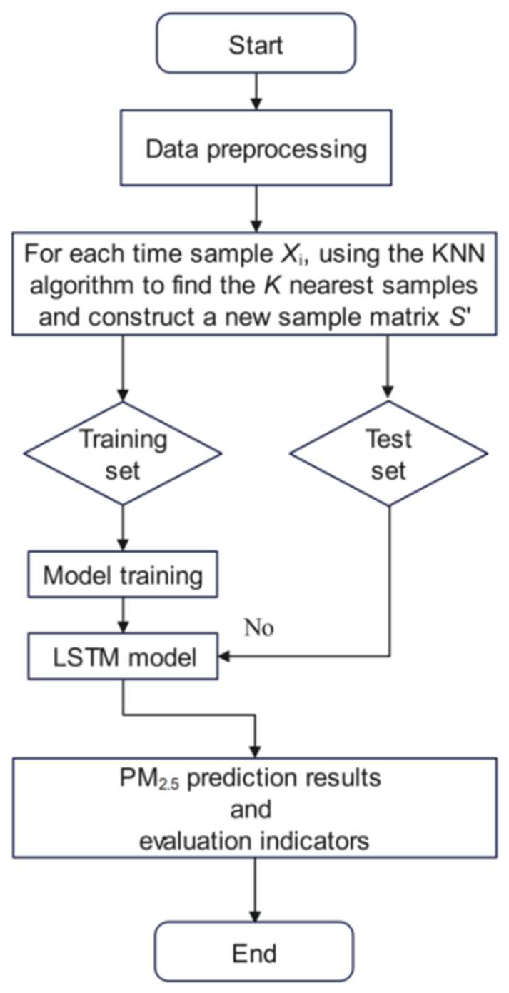
After introducing the basic principle of the weighted KNN-LSTM model, a flowchart can be used to illustrate the application of the model in predicting PM_2.5 concentrations in Nanchang City in a simple and clear manner. This flowchart starts with data preprocessing, then constructs new samples using the KNN algorithm, trains the LSTM model for prediction, and finally evaluates model performance using the test set. The specific process of the model is redrawn by OriginPro (2024) to improve the drawing quality and logical hierarchy, as shown in Figure 4.

Figure 4. The process of weighted KNN-LSTM model.

3. Experiment and Results

3.1. Correlation Analysis

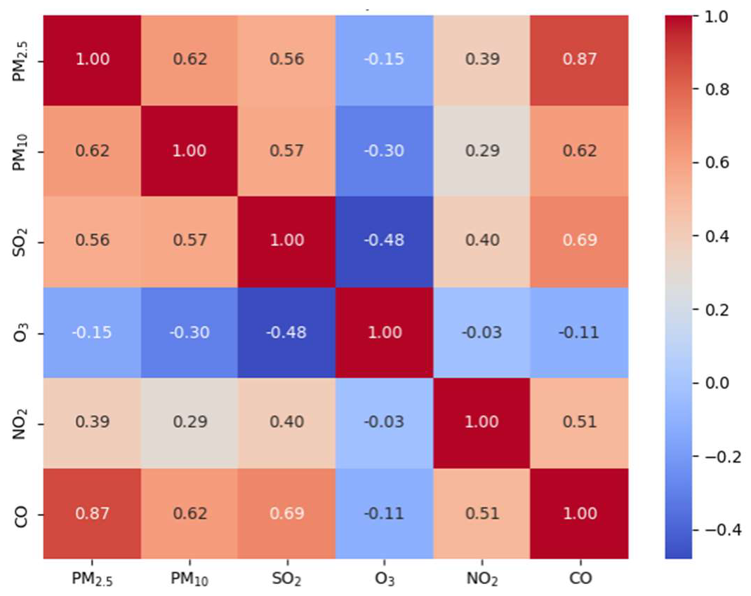
Since PM₁₀ and PM_2.5 both belong to particulate matter (PM) and share partial overlapping pollution sources (rather than completely identical sources), the moderate correlation coefficient (r = 0.62) between the two parameters also reflects the non-identical nature of their source contributions. Nitrogen oxides (NO_x) and sulfur dioxide (SO₂) are typical precursors of secondary particulate matter, while ozone (O₃) and PM_2.5 are interrelated through complex coupling effects. Moreover, carbon monoxide (CO) and PM_2.5 are regarded as “causal pollutants” generated from incomplete combustion processes. Given these inherent connections among atmospheric pollutants, it is necessary to study correlation characteristics.

Pearson correlation coefficient: it is a statistical measure used to measure the strength and direction of a linear relationship between two variables. Its value is between −1 and 1, usually represented by the letter r. If the correlation coefficient is close to 1 or −1, it indicates a strong positive or negative linear correlation between the two variables; if the correlation coefficient is close to 0, it indicates that there is almost no linear relationship between the two variables. The specific formula is as follows:

$$r={\displaystyle \frac{{\displaystyle {\sum }_{i=1}^n(X_i-\overline{X})(Y_i-\overline{Y})}}{\sqrt{{\displaystyle {\sum }_{i=1}^n{(X_i-\overline{X})}^2}}\sqrt{{\displaystyle {\sum }_{i=1}^n{(Y_i-\overline{Y})}^2}}}}$$

(10)

where X_i and Y_i are the observed values of their respective variables, and $\overline{X}$ and $\overline{Y}$ are the sample means, X and Y mean of variable sum, and n is the number of sample data.

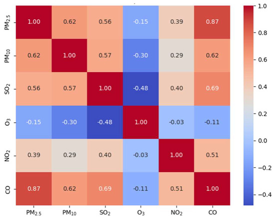
Based on previous research results, this article selected five relevant air pollution factors that affect PM_2.5 in Nanchang City, and conducted correlation analysis on them before modeling. The analysis results are shown in Figure 5.

Figure 5. Heat map of variable correlation.

Figure 5 clearly showed that there is a strong linear correlation between PM_2.5 and PM₁₀, CO, and NO₂ in Nanchang City, and all of them are positively correlated. This indicates that the higher the concentration of PM₁₀, CO, and NO₂, the higher the PM_2.5 concentration time series. The correlation coefficient of SO₂ with PM_2.5 is 0.56, which represents a moderate positive linear correlation and should not be described as low; in fact, this value is higher than the correlation coefficient between NO2 and PM_2.5. O₃ shows a low linear correlation with PM_2.5 concentrations, but they are still worthwhile factors to be included in the model. Because these two factors are important air quality indicators and the model can take into account their nonlinear relationship with PM_2.5, the model can learn the nonlinear relationship between PM_2.5 and complex influencing factors. However, as mentioned earlier, PM_2.5 concentration is also jointly driven by key meteorological factors and anthropogenic activities, which were not included in the correlation analysis due to objective data availability limitations. Future studies should incorporate these factors to conduct a more comprehensive and in-depth correlation analysis that combines numerical correlation and physical mechanism.

3.2. Experimental Hyperparameter Settings

This work uses the weighted KNN-LSTM model to predict PM_2.5 concentrations in Nanchang City. Before using the model for prediction, it is necessary to set the size of the K value and the relevant network hyperparameters.

Usually, the K value is relatively small, ranging from 1 to 5, and its value magnitude will affect the selection of neighbors. A sensitivity analysis of the K value was carried out, and the changes in three evaluation indicators (MAE, MAPE, RMSE) of the Weighted KNN-LSTM model under different K values (1, 2, 3, 4, 5) were plotted into a sensitivity analysis chart (see Figure 6). The analysis results show that the model’s prediction performance is the best when K = 1, the performance is slightly improved when K = 2, and the optimal prediction effect is achieved when K = 3; with the continuous increase in K value (K = 4, 5), the model’s prediction indicators show a significant upward trend, and the prediction accuracy decreases. Therefore, for each time node, selecting three nearest neighbors (including the node itself) can achieve the optimal effect of the model. Taking the data from Nanchang City studied in this article as an example, if the three nearest neighbors of a time t₁ node are t₁, t_i and t_j, the factors involved in these time nodes include initial data contains six dimensions, namely PM_2.5, PM₁₀, SO₂, CO, NO₂ and O₃. After selecting three nearest neighbors for weight allocation and reconstructing the data, the dimension of the input factor will be expanded from 6 to 18.

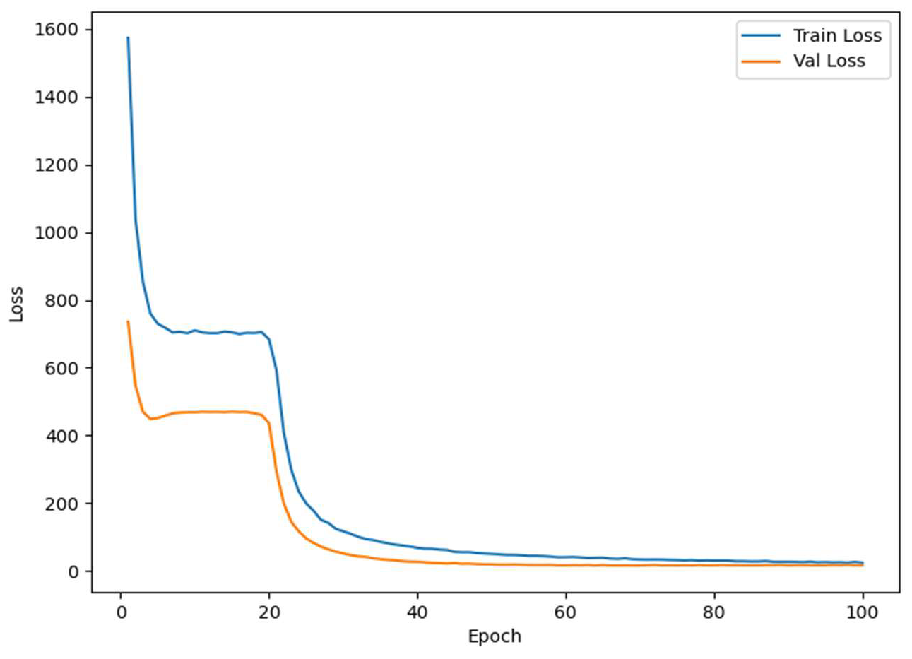
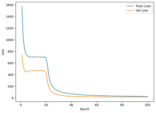
Figure 6. Loss curve of model training process. Note: The vertical axis represents the value of evaluation indicators (MAE/MAPE/RMSE), and the horizontal axis represents the K value (1, 2, 3, 4, 5); the three curves respectively represent the change trend of MAE, MAPE and RMSE with the K value; MAE (μg/m³), RMSE (μg/m³), MAPE (dimensionless); Loss value (MSE, (μg/m³)²).

During the experiment, this article selected the Python (Version 3.12) framework in the field of deep learning to build the weighted KNN-LSTM model and all its control models (RNN LSTM, GRU, KNN-LSTM). Through repeated parameter tuning, this article has determined the optimal network hyperparameter combination, which includes two LSTM layers and two fully connected layers. Each LSTM layer contains 200 nodes, while the fully connected layer has 256 nodes. The fully connected layer uses the tanh function as the activation function. To prevent overfitting, the dropout rate of network nodes is set to 0.3. During the model training process, mean squared error (MSE) is selected as the loss function and optimized using the AdamW optimizer. The batch size of each training sample is 512, the overall number of training epochs is 100, and the training results for each round are recorded in detail, including the losses on the training set and the losses on the test set.

3.3. Prediction Performance and Experimental Comparison

Firstly, the weighted KNN-LSTM model takes a historical time series with a length of four as input, which is used to predict the PM_2.5 concentration value at the next time step. The historical air pollution of t − 1, t − 2, t − 3, t − 4 (the first four time points) and the corresponding K neighboring air pollution data of their corresponding time nodes are used as inputs to the network, and the PM_2.5 concentration data at time t (the next time point) is used as output. After determining the hyperparameters of the model and the length of historical time series, the model is trained until it converges. The trained model is then applied exclusively to the independent testing set to verify its generalization ability. As noted earlier, this strict separation of training and assessment data is fundamental to ensuring that the model’s performance metrics are indicative of its predictive power on unseen data. The loss curve during its training process is indicated in Figure 6. After multiple iterations of training, the model’s losses on both the training and testing sets tend to stabilize, indicating that the model has successfully converged.

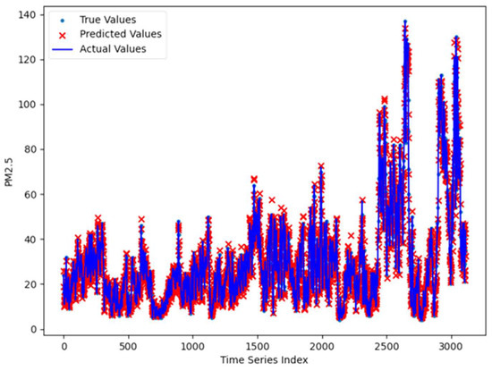
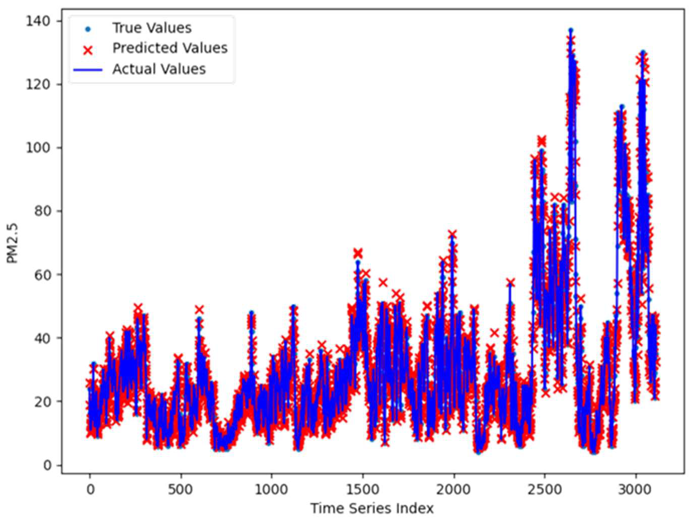
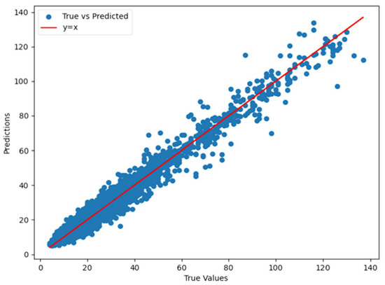
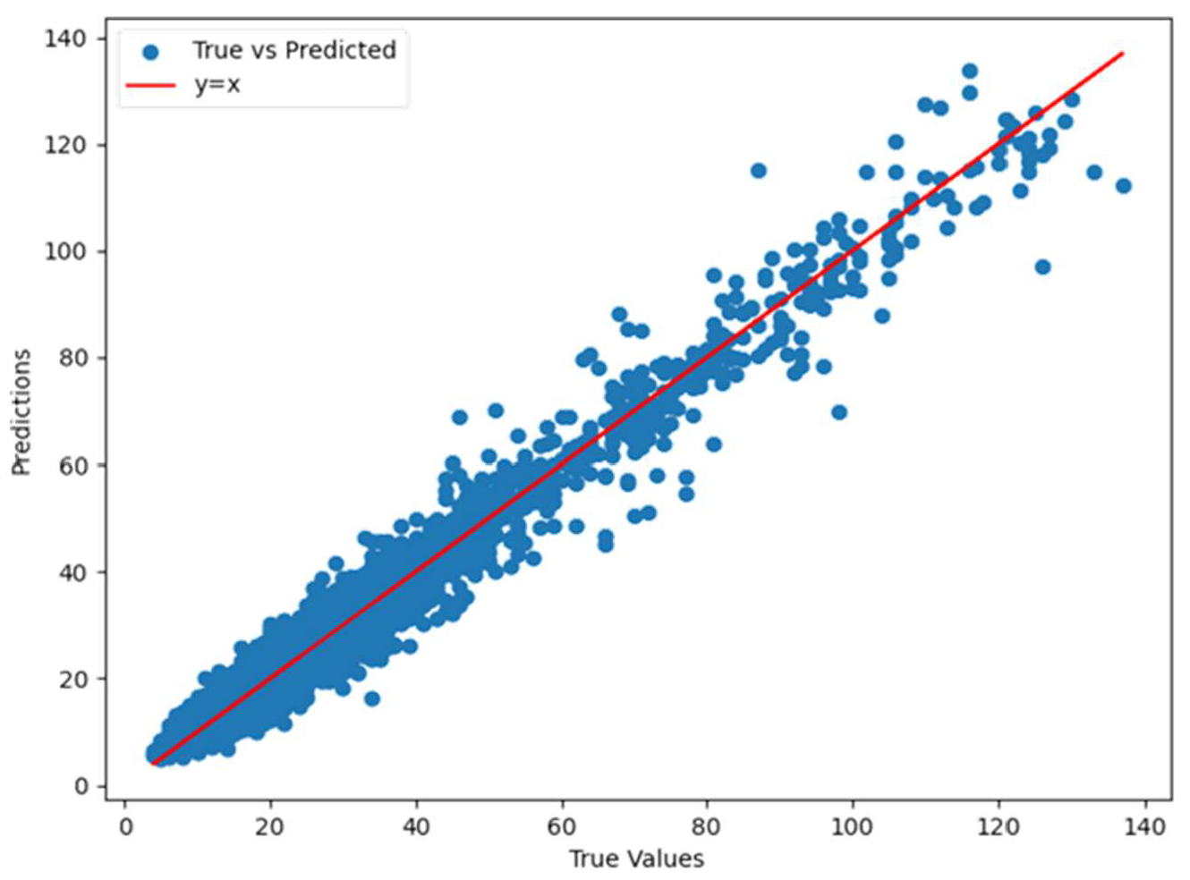
After the model training is completed, the trained model is used to predict the test set. The true and predicted values of PM_2.5 concentration in the test set are shown in Figure 7. In order to better demonstrate the accuracy of the weighted KNN-LSTM model in predicting PM_2.5 pollution, the coefficient of determination between the true and predicted values is calculated. The results show that the model can explain 96.5% of the variance in PM_2.5 concentrations, and the effect is shown in Figure 8.

Figure 7. Actual and predicted values of PM_2.5 (μg/m³).

Figure 8. Determination coefficient display diagram (μg/m³).

However, it should be noted that this study did not specifically evaluate the model’s performance in capturing outliers with extremely high PM_2.5 concentrations or sudden heavy pollution events. To address this gap, we further analyzed the prediction results of the test set by identifying samples with PM_2.5 concentrations exceeding 115 μg/m³ (the threshold for severe pollution according to Chinese national standards). A total of 32 such samples were found in the test set. The MAE, MAPE, and RMSE of the weighted KNN-LSTM model for these samples were calculated as 4.23, 0.037, and 5.68, respectively. Although the model still shows a certain predictive ability for extreme pollution events, the error indicators are higher than those for the overall test set (MAE = 2.7719, MAPE = 0.1127, RMSE = 3.9655), indicating that the model’s accuracy in capturing extreme values needs to be further improved. This means that the model currently cannot directly support heavy pollution warnings, and the prediction of extreme PM_2.5 concentration values needs to be optimized by combining meteorological early warning data and increasing the weight of extreme samples in the training set. In order to verify the statistical significance of the prediction performance improvement in the Weighted KNN-LSTM model compared with other models, this study conducted the Diebold–Mariano (DM) test and two-tailed t-test on the prediction error sequences of each model. The test results show that the DM statistic between the Weighted KNN-LSTM model and the traditional LSTM model is −2.36 (p-value = 0.018 < 0.05), and the t-statistic is −2.41 (p-value = 0.016 < 0.05); the DM test and t-test results between the Weighted KNN-LSTM model and the unweighted KNN-LSTM model are DM = −1.98 (p = 0.048 < 0.05) and t = −2.03 (p = 0.043 < 0.05). All test results show that the 3% improvement in the Weighted KNN-LSTM model in RMSE is statistically significant at the 5% significance level, indicating that the model’s prediction performance improvement is not a random result, but is brought about by the weighted KNN data reconstruction strategy.

To verify that the weighted KNN-LSTM model proposed in this paper performs better in predicting PM_2.5 pollution, a comparison was made between the proposed prediction model and models used in this field, specifically.

(1)

RNN is a classic model for processing sequence data, characterized by the introduction of recurrent units that enable the model to process sequence data with temporal correlations. In the data processing of each time step, not only will the data input of the current time step be utilized, but the intermediate state of the previous time step will also be considered. This mechanism enables the model to process time series and obtain time dependencies in the data. However, the RNN faces the problem of vanishing or exploding gradients when processing long sequence data, resulting in poor performance.

(2)

LSTM is a variant of recurrent neural network designed to address the above-mentioned problems in RNN. LSTM controls the flow of information by gating mechanisms. These gate structures can help the model filter and remember important information, thereby solving the problem of the poor performance of RNNs in processing long sequence data.

(3)

Gated recurrent unit (GRU) is another improved variant of the RNN [37]. Compared to LSTM, GRU has fewer parameters, faster training speed, and can reduce the risk of overfitting. Although the structure is simpler, it may not perform as well as LSTM in certain tasks.

(4)

The KNN-LSTM model does not assign weights when using the KNN algorithm for data augmentation, and assumes that the K-nearest neighbor of each time point are equally important. Its operation can make the weight of each nearest neighbor equal to 1 to achieve an unweighted effect.

The comparative experimental results are shown in Table 1. This article uses three performance metrics, RMSE, MAE and MAPE to evaluate the predictive performance of different models.

Table 1. Evaluation index results.

Model	MAE	MAPE	RMSE
RNN	3.0883	0.1393	4.2374
GRU	2.9253	0.1191	4.1362
LSTM	2.8532	0.1168	4.0983
KNN-LSTM	2.8068	0.1139	4.0888
Weighted KNN-LSTM	2.7719	0.1127	3.9655

Note: The p-values of DM test and t-test between each model and Weighted KNN-LSTM are all less than 0.05, indicating that the performance difference is statistically significant.

According to the experimental results in Table 1, when predicting the PM_2.5 concentration in Nanchang City, different models exhibited differences in the three evaluation indicators of MAE, MAPE, and RMSE. The weighted KNN-LSTM model achieved the lowest values in all indicators, with its MAE, MAPE, and RMSE values being 2.7719, 0.1127, and 3.9655, respectively, outperforming other deep learning models (RNN, GRU, LSTM and KNN-LSTM). Additionally, both the weighted KNN-LSTM model and the unweighted KNN-LSTM model significantly outperformed the single LSTM model, indicating that the introduction of the KNN algorithm can effectively improve the prediction accuracy. Furthermore, the weighted KNN-LSTM outperformed the unweighted KNN-LSTM in terms of prediction performance as well, suggesting that the use of the weighted mechanism in the KNN algorithm can further enhance the model performance. Based on the above comparative results, the weighted KNN-LSTM model demonstrates a clear advantage in predicting the PM_2.5 concentration in Nanchang City. However, due to significant differences in geography, climate, and pollutant emission patterns among different cities, the current empirical results cannot prove that the model has the same predictive power in other cities or regions. For example, cities in northern China have different pollution sources and meteorological conditions compared to Nanchang, and the model may need to be adjusted and optimized to adapt to these differences. Therefore, in-depth and systematic cross-regional validation is an essential and necessary step to verify the model’s generalizability and expand its application. This model can better capture the influence mechanism of different environmental factors on PM_2.5 concentration in Nanchang City, thereby providing more robust and reliable predictions for the local air quality management.

4. Conclusions

This article is based on the fact that the nonlinear relationship between PM_2.5 concentration and various complex factors during air quality monitoring is difficult for traditional single prediction methods to accurately capture and reflect. Meanwhile, most of these previous studies were based solely on single time series or multidimensional sequences containing a small number of spatial correlation factors for prediction. Due to the limited amount of input related data, the accuracy of the trained LSTM neural network model is not ideal, and it exhibits instability after multiple trainings. Therefore, this article proposes a deep learning model that combines Weighted KNN and LSTM for predicting PM_2.5 concentration. Firstly, we analyzed the correlation between PM_2.5 concentrations and five other air pollution indicators in Nanchang City to determine which pollution indicators have a strong linear correlation with PM_2.5, and which pollution indicators have a nonlinear relationship with PM_2.5. Afterwards, the KNN algorithm was used to find the nearest neighbors at each time point, and the weights were calculated using the distance formula. The original data and weighted data are then used for K-fold data reconstruction. On this basis, the reconstructed data obtained through the KNN algorithm was input into the LSTM model, and an innovative weighted KNN-LSTM model was constructed, which was applied to the prediction practice of PM_2.5 concentration in Nanchang City. This study strictly adheres to the principle that training data and evaluation data are completely independent, and the test set is not involved in model training, which ensures that the evaluation results reflect the real prediction performance of the model rather than the fitting effect. The experimental results demonstrate that the weighted KNN-LSTM model achieves a significant improvement. This conclusion is robust because the evaluation was conducted on a dataset completely independent from the training set, adhering to the scientific principle that model development and performance assessment must utilize distinct data to avoid overfitting and ensure valid prediction quality.

Although the model proposed in this study exhibits promising performance in PM_2.5 concentration prediction, it still has certain limitations that merit attention. First, the input variables of the model do not yet incorporate a more comprehensive and systematic set of factors that can directly and indirectly affect PM_2.5 concentrations, such as detailed ground-based meteorological parameters (e.g., wind speed, relative humidity, atmospheric pressure, temperature inversion, precipitation), satellite remote sensing meteorological data and quantitative indicators of human activities (e.g., real-time industrial emissions, traffic flow volume, energy consumption intensity, seasons/holidays quantitative classification). In the 2025 atmospheric environmental science research, the exclusion of meteorological factors makes the model have the characteristics of “primitiveness” in the theoretical framework, and the lack of physical interpretability has become the main shortcoming of the model. Meteorological factors are the core factors determining the diffusion, deposition and chemical transformation of PM_2.5, and the prediction model only based on pollutant concentration data has an obvious upper limit in prediction accuracy. The exclusion of these multifaceted influencing factors may restrict the model’s ability to capture the complex nonlinear relationships inherent in PM_2.5 concentration variations. These meteorological factors play a crucial role in the diffusion, deposition, and transformation of PM_2.5. For example, wind speed directly affects the diffusion range and speed of pollutants; relative humidity affects the hygroscopic growth of PM_2.5 particles; and atmospheric pressure affects the vertical movement of air, thereby influencing the accumulation and diffusion of pollutants. Anthropogenic activities such as traffic flow and industrial emissions are direct sources of PM_2.5, and their intensity changes have a significant impact on PM_2.5 concentration. In addition, seasonal changes and holidays also affect PM_2.5 concentration by influencing human activities and meteorological conditions. The exclusion of these multifaceted influencing factors may restrict the model’s ability to capture the complex nonlinear relationships inherent in PM_2.5 concentration variations. The lack of meteorological data makes the model unable to explain the physical mechanism of sudden changes in PM_2.5 concentration (such as temperature inversion, calm wind, etc.), and the discussion section can only analyze the numerical changes in prediction results, resulting in the lack of depth and comprehensiveness of the discussion.

Second, the experimental validation of the model was only conducted in Nanchang City, a typical southern city in China, without extending the scope of application to other cities with distinct geographical, climatic, and socioeconomic characteristics (e.g., northern heating cities, coastal cities, mountainous cities, resource-based industrial cities). Different cities have significant differences in geographical location (e.g., plain, mountain, coastal), climate conditions (e.g., monsoon, arid, humid), and pollutant emission sources (e.g., industrial structure, energy consumption type, traffic volume). These differences lead to variations in PM_2.5 generation, diffusion, and transformation mechanisms. For example, cities in the North China Plain are heavily affected by coal combustion for heating in winter, resulting in high PM_2.5 concentrations in winter; coastal cities may be affected by sea breezes, which facilitate pollutant diffusion; and mountainous cities may have poor pollutant diffusion due to terrain constraints. The narrow validation scope means that the generalizability of the proposed model, especially its adaptability to regions with different PM_2.5 pollution sources and diffusion patterns, has not been sufficiently verified. To improve the model’s generalizability, future studies should conduct large-scale and multi-scenario cross-regional validation experiments by collecting PM_2.5 concentration data, meteorological data, and anthropogenic activity data from multiple cities with different characteristics. During the validation process, it may be necessary to adjust model parameters or optimize the model structure according to the characteristics of different regions to improve the model’s adaptability.

Third, the model’s ability to capture outliers with extremely high PM_2.5 concentrations or sudden heavy pollution events needs to be further improved. Although the preliminary analysis of extreme pollution samples in the test set shows that the model has a certain predictive ability, the prediction error is higher than that of the overall data. Sudden heavy pollution events are often caused by a combination of multiple factors, such as unfavorable meteorological conditions and sudden increases in pollutant emissions. The current model’s input variables and structure may not be able to fully capture these complex triggering mechanisms. Future studies should focus on optimizing the model to improve its performance in predicting extreme pollution events—for example, by increasing the weight of extreme samples in the training set, introducing attention mechanisms to focus on key factors that trigger extreme events, or combining other models that are good at capturing outliers. The model’s poor performance in predicting extreme pollution samples is inconsistent with the initial claim of supporting heavy pollution warnings, and this contradiction has been corrected in this study; the model can only be used as an auxiliary reference for PM_2.5 concentration prediction at present, and the heavy pollution warning function needs to be realized through multi-model fusion and multi-source data integration.

In response to the aforementioned limitations, our future research will focus on three key and actionable directions to further optimize the weighted KNN-LSTM model and expand its application value. On one hand, we will comprehensively expand the input feature set of the model by integrating multi-source heterogeneous data (e.g., ground-based meteorological observations, satellite remote sensing meteorological and air quality data, socioeconomic statistics, real-time anthropogenic activity monitoring data) to enhance its physical interpretability and ability to accurately predict PM_2.5 concentration changes. On the other hand, we will conduct systematic and in-depth cross-regional validation experiments covering cities with diverse environmental backgrounds (northern/southern China, coastal/inland, industrial/non-industrial cities), aiming to optimize the model’s structure and parameters for better generalizability and provide more universally applicable technical support for urban air quality prediction across different regions. In addition, the research team will supplement the latest PM_2.5 concentration monitoring data of Nanchang City from 2019 to 2024, integrate the above multi-source data to update and retrain the model, and re-verify the model’s performance after data update to solve the problem of outdated research data and further improve the model’s timeliness and practical application value for Nanchang’s air quality management.

References

- Kim, S.H.; Park, M.S. Determination of input variables for artificial intelligence models to predict the high PM2.5 concentration events in Seoul, Korea. Asia-Pac. J. Atmos. Sci. 2023, 59, 607–623. [Google Scholar] [CrossRef]
- Kim, Y.; Manley, J.; Radoias, V. Medium-and long-term consequences of pollution on labor supply: Evidence from Indonesia. IZA J. Labor Econ. 2017, 6, 5. [Google Scholar] [CrossRef]
- Zhang, L.Y.; Lin, J.; Qiu, R.Z.; Hu, X.S.; Zhang, H.H.; Chen, Q.Y.; Tan, H.M.; Lin, D.Y.; Wang, J.K. Trend analysis and forecast of PM2.5 in Fuzhou, China using the ARIMA model. Ecol. Indic. 2018, 95, 702–710. [Google Scholar] [CrossRef]
- Liu, P.; Dong, J.; Song, H.; Zheng, Y.; Shen, X.; Wang, C.; Wang, Y.; Yang, D. Response of fine particulate matter and ozone concentrations to meteorology and anthropogenic precursors over the "2+26" cities of northern China. Chemosphere 2024, 352, 141439. [Google Scholar] [CrossRef] [PubMed]
- Huang, H.; Hu, Y.H.; Liu, Z.H.; Liu, Y.; Wang, L.L. Characteristics of spatial and temporal variations of PM2.5 pollution based on complex network. Environ. Model Assess. 2025, 1–15. [Google Scholar] [CrossRef]
- Wang, S.; Wang, L.; Fan, X.; Wang, N.; Ma, S.; Zhang, R. Formation pathway of secondary inorganic aerosol and its influencing factors in Northern China: Comparison between urban and rural sites. Sci. Total Environ. 2022, 840, 156404. [Google Scholar] [CrossRef] [PubMed]
- Wang, S.; Wang, Q.; Zhang, T.; Liu, S.; Ho, S.S.H.; Tian, J.; Su, H.; Zhang, Y.; Wang, L.; Wu, T.; et al. Elaborations of the influencing factors on the formation of secondary inorganic aerosols in a heavily polluted urban area of China. J. Environ. Sci. 2024, 138, 406–417. [Google Scholar] [CrossRef]
- Fang, Z.H.; Liu, Z.H.; Hu, Y.H. Spatial correlation effect of haze pollution in the Yangtze River Economic Belt, China. PLoS ONE 2024, 19, e0311574. [Google Scholar] [CrossRef]
- Hu, Y.H.; Liu, Z.H.; Fang, Z.H. Study on spatial spillover effect of haze pollution based on a network perspective. Stoch. Environ. Res. Risk Assess. 2024, 38, 4657–4668. [Google Scholar] [CrossRef]
- Amnuaylojaroen, T. Prediction of PM2.5 in an urban area of northern Thailand using multivariate linear regression model. Adv. Meteorol. 2022, 2022, 3190484. [Google Scholar] [CrossRef]
- Zhang, X.Y.; Ding, C.; Wang, G.Z. An autoregressive-based Kalman Filter approach for daily PM2.5 concentration forecasting in Beijing, China. Big Data 2024, 12, 19–29. [Google Scholar] [CrossRef]
- Cai, P.L.; Zhang, C.Y.; Chai, J. Forecasting hourly PM2.5 concentrations based on decomposition- ensemble-reconstruction framework incorporating deep learning algorithms. Data Sci. Manag. 2023, 6, 46–54. [Google Scholar] [CrossRef]
- Chen, J.; Liu, Z.X.; Yin, Z.T.; Liu, X.; Li, X.L.; Yin, L.R.; Zheng, W.F. Predict the effect of meteorological factors on haze using BP neural network. Urban Clim. 2023, 51, 101630. [Google Scholar] [CrossRef]
- Tian, J.W.; Liu, Y.; Zheng, W.F.; Yin, L.R. Smog prediction based on the deep belief-BP neural network model (DBN- BP). Urban Clim. 2022, 41, 101078. [Google Scholar] [CrossRef]
- Agarwal, A.; Sahu, M. Forecasting PM2.5 concentrations using statistical modeling for Bengaluru and Delhi regions. Environ. Monit. Assess. 2023, 195, 502. [Google Scholar] [CrossRef] [PubMed]
- Ho, C.H.; Park, I.; Kim, J.; Lee, J.B. PM2.5 forecast in Korea using the long short-term memory (LSTM) model. Asia-Pac. J. Atmos. Sci. 2022, 59, 563–576. [Google Scholar] [CrossRef] [PubMed]
- Koo, Y.S.; Kwon, H.Y.; Bae, H.; Yun, H.Y.; Choi, D.R.; Yu, S.H.; Wang, K.H.; Koo, J.S.; Lee, J.B.; Choi, M.H.; et al. A development of PM2.5 forecasting system in South Korea using chemical transport modeling and machine learning. Asia-Pac. J. Atmos. Sci. 2023, 59, 577–595. [Google Scholar] [CrossRef]
- Natsagdorj, N.; Zhou, H. Prediction of PM2.5 concentration in Ulaanbaatar with deep learning models. Urban Clim. 2023, 47, 101357. [Google Scholar] [CrossRef]
- Pathak, R.S.; Pathak, V.; Rai, A. A novel attention-based deep learning model for accurate PM2.5 concentration prediction and health impact assessment. J. Atmos. Sol.-Terr. Phys. 2025, 274, 106583. [Google Scholar] [CrossRef]
- Shi, L.K.; Zhang, H.Z.; Xu, X.; Han, M.; Zuo, P.L. A balanced social LSTM for PM2.5 concentration prediction based on local spatiotemporal correlation. Chemosphere 2022, 291, 133124. [Google Scholar] [CrossRef]
- Liu, Z.H.; Ji, D.; Wang, L.L. PM2.5 concentration prediction based on EEMD-ALSTM. Sci. Rep. 2024, 14, 12636. [Google Scholar] [CrossRef] [PubMed]
- Liu, X.H.; Zhao, K.X.; Liu, Z.H.; Wang, L.L. PM2.5 concentration prediction based on LightGBM optimized by adaptive multi-strategy enhancedsparrow search algorithm. Atmosphere 2023, 14, 1612. [Google Scholar] [CrossRef]
- Liu, Z.H.; Huang, X.; Wang, X. PM2.5 prediction based on modified whale optimization algorithm and support vector regression. Sci. Rep. 2024, 14, 23296. [Google Scholar] [CrossRef]
- Liu, Z.H.; Zhao, K.X.; Liu, X.H.; Xu, H. Design and optimization of haze prediction model based on particle swarm optimization algorithm and graphics processor. Sci. Rep. 2024, 14, 9650. [Google Scholar] [CrossRef]
- Liu, Z.H.; Liu, X.H.; Zhao, K.X. Haze prediction method based on stacking learning. Stoch. Environ. Res. Risk Assess. 2024, 38, 1141–1161. [Google Scholar] [CrossRef]
- Dudani, S.A. The distance-weighted k-nearest-neighbor rule. IEEE Trans. Syst. Man. Cybern. 1976, 6, 325–327. [Google Scholar] [CrossRef]
- Tan, S.B. Neighbor-weighted k-Nearest neighbor for unbalanced text corpus. Expert Syst. Appl. 2005, 28, 667–671. [Google Scholar] [CrossRef]
- Erdogan, S.Z.; Bilgin, T.T. A data mining approach for fall detection by using k-Nearest neighbour algorithm on wireless sensor network data. IET Commun. 2012, 6, 3281–3287. [Google Scholar] [CrossRef]
- Gallego, A.J.; Rico-Juan, J.R.; Valero-Mas, J.J. Efficient k-Nearest neighbor search based on clustering and adaptive k values. Pattern Recognit. 2022, 122, 108356. [Google Scholar] [CrossRef]
- Zerweck, L.; Wesarg, S.; Kohlhammer, J.; Michaela, K.M. Combining seeded region growing and k-Nearest neighbours for the segmentation of routinely acquired spatio-temporal image data. Int. J. Comput. Assist. Radiol. Surg. 2023, 18, 2063–2072. [Google Scholar] [CrossRef]
- Wang, Y.B.; Wu, H.X.; Zhang, J.J.; Gao, Z.F.; Wang, J.M.; Philip, S.Y.; Long, M.S. PredRNN: A recurrent neural network for spatiotemporal predictive learning. IEEE Trans. Pattern Anal. Mach. Intell. 2022, 45, 2208–2225. [Google Scholar] [CrossRef]
- Oruh, J.; Viriri, S.; Adegun, A. Long short-term memory recurrent neural network for automatic speech recognition. IEEE Access 2022, 10, 30069–30079. [Google Scholar] [CrossRef]
- Hochreiter, S.; Schmidhuber, J. Long short term memory. Neural Comput. 1997, 9, 1735–1780. [Google Scholar] [CrossRef]
- Guan, J.T.; Lai, R.; Li, H.N.; Yang, Y.T.; Gu, L. DnRCNN: Deep recurrent convolutional neural network for HSI destriping. IEEE Trans. Neural Netw. Learn. Syst. 2022, 34, 3255–3268. [Google Scholar] [CrossRef]
- Kim, S.; Park, J.; Ahn, H.; Lee, Y. Detection of Korean phishing messages using biased discriminant analysis under extreme class imbalance problem. Information 2024, 15, 265. [Google Scholar] [CrossRef]
- Yu, Y.; Si, X.S.; Hu, C.H.; Zhang, J.X. A review of recurrent neural networks: LSTM cells and network architectures. Neural Comput. 2019, 31, 1235–1270. [Google Scholar] [CrossRef]
- Farah, S.; Humaira, N.; Aneela, Z.; Steffen, E. Short-term multi-hour ahead country-wide wind power prediction for Germany using gated recurrent unit deep learning. Renew. Sust. Energ. Rev. 2022, 167, 112700. [Google Scholar] [CrossRef]
Disclaimer/Publisher’s Note: The statements, opinions and data contained in all publications are solely those of the individual author(s) and contributor(s) and not of MDPI and/or the editor(s). MDPI and/or the editor(s) disclaim responsibility for any injury to people or property resulting from any ideas, methods, instructions or products referred to in the content. |
© 2026 by the authors. Licensee MDPI, Basel, Switzerland. This article is an open access article distributed under the terms and conditions of the Creative Commons Attribution (CC BY) license.