


Abstract
India faces severe PM2.5–O3 compound pollution, and the 2023 G20 Summit in New Delhi provided a valuable case for examining how short-term emission controls interact with unfavorable late-monsoon meteorology. In this study, the WRF-CMAQ modeling system was applied to quantify the relative contributions of meteorological variability and graded multisectoral emission controls to PM2.5 and ozone changes during the summit period. The results show that both pollutants exhibited clear stage-dependent variations, with lower concentrations during the summit and rapid rebound afterward. Relative to the 2022 meteorology sensitivity case, the 2023 meteorological background increased PM2.5 by 6.76 μg/m3 and MDA8 O3 by 4.37 ppb over New Delhi, indicating a distinct meteorological penalty during the monsoon withdrawal period. Under progressively strengthened control scenarios, PM2.5 declined from 79.01 to 66.35 μg/m3, while MDA8 O3 decreased from 81.19 to 77.67 ppb. The strongest control scenario reduced PM2.5 more than the meteorological penalty and substantially mitigated the ozone enhancement, although it did not fully offset the adverse meteorological effect on O3. These findings demonstrate that high-intensity coordinated controls can effectively alleviate PM2.5–O3 compound pollution even under unfavorable meteorological conditions.
1. Introduction
India experiences some of the most severe air pollution in the world, with both fine particulate matter (PM2.5) and ozone (O3) posing substantial risks to public health and sustainable development [1,2]. In recent years, PM2.5–O3 compound pollution has become an increasingly important air-quality challenge across India, particularly over the Indo-Gangetic Plain, where high particulate loading and active photochemical pollution frequently coexist [3,4]. New Delhi, as one of the major urban centers in this region, is characterized by persistently high PM2.5 concentrations and elevated ozone levels, making it a representative hotspot for studying complex air pollution in South Asia [5,6].
The 2023 G20 Summit in New Delhi provided a valuable natural experiment for investigating the atmospheric response to short-term emission controls. During the summit period, multiple administrative control measures were implemented, including restrictions on traffic, industrial activities, and construction-related emissions [7,8]. Such high-intensity short-term interventions can offer an opportunity to evaluate how rapidly air quality responds to coordinated emission reductions [9,10]. However, the summit took place during the monsoon withdrawal period in September, when rainfall weakens, wet scavenging decreases, and atmospheric dispersion conditions begin to deteriorate over northern India [4,11]. Under such conditions, it is difficult to distinguish whether observed or simulated air-quality changes are primarily driven by emission controls or by meteorological variability [12].
Previous air-quality modeling studies over India have substantially improved our understanding of PM2.5 distributions, sectoral emissions, and source contributions [13,14,15]. Recent work has also emphasized the importance of updated emission inventories, rigorous model evaluation, and regional source attribution for interpreting India’s air pollution patterns [14]. However, most existing studies have focused on annual or seasonal mean pollution, long-term source attribution, or single-pollutant behavior, while fewer studies have quantitatively examined the relative roles of unfavorable meteorology and graded short-term emission controls during a major event, especially from a PM2.5–O3 co-control perspective [3,16]. In particular, it remains unclear to what extent adverse late-monsoon meteorological conditions enhanced PM2.5 and O3 during the 2023 G20 period, whether graded control strategies could offset this meteorological penalty, and why PM2.5 and O3 responded differently to the same short-term interventions [17]. This study moves beyond conventional event-based attribution by explicitly quantifying the competition between meteorological penalty and emission-control benefits, thereby providing a process-oriented framework for understanding PM2.5–O3 co-response under unfavorable atmospheric conditions.
In this study, we applied the WRF-CMAQ modeling system to investigate the relative roles of meteorology and coordinated short-term emission controls in shaping PM2.5 and O3 pollution during the 2023 G20 Summit in New Delhi. Using a baseline scenario, a meteorological sensitivity scenario, and three graded emission-control scenarios, we examined (1) the stage-dependent evolution of PM2.5 and O3 during the summit period, (2) the meteorological penalty associated with the monsoon withdrawal background, and (3) the effectiveness of coordinated multisectoral controls in reducing PM2.5 and O3 under unfavorable atmospheric conditions. This study aims to provide a quantitative basis for understanding PM2.5–O3 co-response during major events and to offer scientific support for short-term air-quality management in India and other developing regions facing similar challenges.
2. Materials and Methods
2.1. Model Configuration and Study Domain
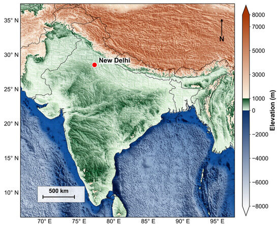
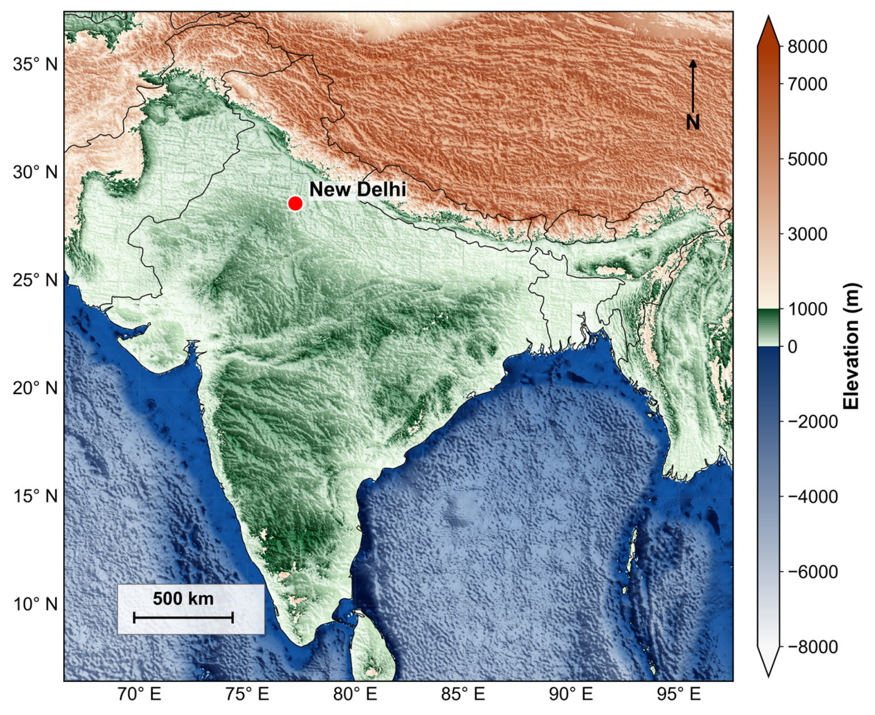
The Weather Research and Forecasting model (WRF, version 4.1.2) coupled with the Community Multiscale Air Quality model (CMAQ, version 5.0.2) was applied to simulate air quality over India. The modeling domain, illustrated in Figure 1, covered the Indian subcontinent with a horizontal resolution of 36 km × 36 km (comprising 117 × 117 grid cells) under a Lambert conformal projection. Eighteen vertical sigma layers were used, with enhanced resolution near the surface to better represent boundary-layer processes. Meteorological fields were generated by WRF using NCEP FNL reanalysis data as initial and boundary conditions. The WRF outputs were then processed to provide the meteorological inputs required by CMAQ. These inputs include temperature, wind speed and direction, relative humidity, pressure, planetary boundary layer height, precipitation, cloud fields, and other variables governing transport, turbulent mixing, deposition, and chemical transformation. For chemical transport, the SAPRC-11 gas-phase mechanism [18] and the AERO6 aerosol module [19,20] were adopted in CMAQ to represent the formation and evolution of PM2.5 and O3 under the high-emission background of India. These model settings were selected to provide a consistent framework for evaluating regional pollution characteristics and the short-term air-quality response during the 2023 G20 Summit.
Figure 1.
The simulation domain has a horizontal resolution of 36 km. The elevation data are collected from ETOPO2v2 (https://www.ngdc.noaa.gov/mgg/global/relief/ETOPO2/ETOPO2v2-2006/ETOPO2v2c/ (accessed on 19 April 2026)) at the resolution of 2′.
2.2. Emission Inventories and Scenario Design
Anthropogenic emissions were primarily based on the EDGAR v8.1 inventory (https://edgar.jrc.ec.europa.eu/dataset_ap81 (accessed on 3 March 2026)) [21]. Source category profiles are extracted from SPECIATE 4.3, a speciation profile database developed by the US EPA [22,23]. To construct a representative 2023 emission field, the 2022 baseline emissions were updated using sector-specific scaling factors derived from socioeconomic activity data. As shown in Table S1, the scaling factors were set as 1.11 for on-road transport (based on vehicle registration and fuel consumption growth from FADA), 1.07 for energy, industry, and off-road sources (based on GDP growth and industrial production index from MoSPI), and 1.008 for agriculture and residential sources (based on population growth from World Bank). This approach retained the spatial pattern of EDGAR v8.1 while updating the total emissions to 2023 levels. Such an approach is widely adopted in large-scale air-quality modeling studies when near-real-time sector-specific emission inventories are unavailable [24,25]. Biogenic and biomass-burning emissions were represented using MEGAN v2.1 [26] and FINN v2.5 [27,28]. The emission inputs applied in CMAQ included anthropogenic emissions from EDGAR v8.1 (chemically speciated using SPECIATE 4.3), biogenic emissions from MEGAN v2.1, and biomass-burning emissions from FINN v2.5. These datasets provided the gridded emission inputs required by the SAPRC-11/AERO6 chemical mechanism.
To quantify the relative roles of meteorology and short-term administrative controls during the G20 period, a set of controlled scenarios were designed. The baseline scenario S2 used 2023 meteorology and 2023 emissions. The meteorological sensitivity scenario S3 was not intended to represent an actual emission-meteorology combination in a specific year. Instead, it was designed as a controlled sensitivity experiment: the 2023 emission field was kept identical to S2, while only the meteorological fields were replaced by those from September 2022. Thus, emissions remained identical between S2 and S3, and the S2–S3 difference allows us to quantify the effective contribution of meteorological variability between 2023 and 2022 [16,29]. Three graded control scenarios were further constructed using the 2023 baseline as the reference: S4-A applied emission reductions of 20% for road traffic and 15% for construction and road dust; S4-B applied reductions of 40% for road traffic, 30% for construction and road dust, and 15% for industrial point sources; and S4-C applied reductions of 60%, 50%, and 30% to these three source categories, respectively. These scenarios were designed to represent progressively strengthened short-term interventions during the summit period and to evaluate whether stronger multisectoral controls could offset the unfavorable meteorological background. These three sectors were selected because they correspond to the main source categories that can be directly affected by short-term administrative measures during major events [9,30]. During the G20 Summit, temporary interventions in Delhi mainly involved traffic restrictions, suspension or reduction in construction-related activities, and controls on industrial operations. Therefore, on-road traffic, construction and road dust, and industrial point sources were chosen to represent the most policy-relevant and rapidly adjustable emission sectors. An additional 2022 baseline scenario (S1) was also conducted in the broader thesis framework for annual comparison, but the present paper focuses on S2, S3, and S4-A/B/C during the 2023 G20 period. The main model configuration is summarized in Table S2, and the scenario design is listed in Table 1.
Table 1.
Scenario design.
2.3. Observational Data and Model Evaluation
Ground-based air-quality observations were obtained from the Central Pollution Control Board (CPCB) monitoring network in India (https://airquality.cpcb.gov.in/ccr/ (accessed on 12 April 2026)). Model performance was evaluated against observed PM2.5 and O3 concentrations for 2023 using commonly used statistical metrics, including observed mean, predicted mean, mean fractional bias (MFB), and mean fractional error (MFE) [31]. MFB and MFE were selected as the primary performance metrics because they are normalized indicators commonly used in air-quality model evaluation and allow model bias and error to be compared across pollutants and spatial scales. The evaluation was conducted at both the broader regional scale and the New Delhi urban scale in order to ensure that the model could reasonably reproduce the pollution levels and temporal variability relevant to the G20 case study. Since the main objective of this work is to quantify relative changes among scenarios rather than to exactly reproduce every hourly concentration value, the model evaluation was primarily used to establish a reliable baseline for subsequent attribution analyses.
2.4. Attribution Framework and Data Analysis
To analyze the evolution of air pollution during the summit, the period from 1 to 15 September 2023 was divided into three stages: pre-G20 (1–7 September), during-G20 (8–10 September), and post-G20 (11–15 September). Temporal evolution, stage statistics, and spatial differences were then examined for PM2.5 and MDA8 O3. As S2 and S3 share the same 2023 emission field, the meteorological penalty was quantified as the concentration difference between S2 and S3 under identical emissions, whereas the control benefit was quantified as the difference between each control scenario (S4-A, S4-B, or S4-C) and the baseline scenario S2. It should be noted that the S2–S3 difference represents an effective meteorological contribution under fixed emissions, rather than a fully decoupled physical attribution, because meteorology and atmospheric chemistry remain nonlinearly coupled in the model framework. Spatial difference maps were generated to examine the regional distribution of meteorological and control effects [32]. The HCHO/NO2 ratio was calculated over the 3 × 3 grid cells surrounding New Delhi as an indicator of the O3 chemical sensitivity regime [33,34]. In addition, the responses of major PM2.5 components, including sulfate, nitrate, ammonium, SOA, and Primary PM, were analyzed under the graded control scenarios in order to identify the dominant contributors to particulate-matter reduction. For the event-period analysis, pollutant concentrations over New Delhi were calculated using the administrative-region mean, so that all scenario comparisons in the summit case study were based on a consistent spatial definition.
3. Results
3.1. Model Performance
The WRF v4.1.2 meteorological fields were first evaluated against surface observations. Key variables, including 2 m temperature (T2), 10 m wind speed (WS), wind direction (WD), and relative humidity (RH), were quantitatively evaluated using statistical metrics, including mean bias (MB), gross error (GE), and root-mean-square error (RMSE), following commonly used meteorological model performance benchmarks [35]. The detailed results are provided in Table S3. Overall, WRF reproduced the major meteorological conditions over India with reasonable stability. T2, WS, and RH showed generally acceptable performance for regional-scale air-quality modeling, while larger uncertainties were found for WD, especially in GE and RMSE. This limitation is commonly reported in regional simulations over complex terrain and monsoon-affected regions, partly because the 36 km horizontal resolution smooths sub-grid terrain and land-surface heterogeneity, and because wind direction errors can be amplified under low-wind-speed conditions [13,25]. Nevertheless, the MB values for WS and WD during September, the key month for the G20 analysis, remained relatively small. Therefore, the meteorological fields were considered adequate for driving the subsequent CMAQ simulations and for supporting the scenario-based attribution analysis.
As shown in Table 2, the WRF-CMAQ modeling framework was evaluated against CPCB observations for 2023 to assess its ability to reproduce the major characteristics of PM2.5 and O3 over India and, more specifically, over New Delhi. At the regional scale, the model reproduced the overall levels of both pollutants reasonably well. For 2023, the observed and simulated annual mean PM2.5 concentrations were 56.98 and 60.71 μg/m3, respectively, with a mean fractional bias (MFB) of −0.05 and a mean fractional error (MFE) of 0.65. The negative MFB indicates an underestimation of PM2.5, which may be associated with uncertainties in local emissions and the smoothing of urban pollution hotspots at the 36 km model resolution. For O3, the observed and simulated annual mean concentrations were 68.52 and 82.36 ppb, respectively, with an MFB of 0.19 and an MFE of 0.38. While the PM2.5 simulation met the recommended criteria for acceptable performance, O3 was moderately overestimated, with its normalized bias and error exceeding the ideal EPA performance targets [36]. This discrepancy reflects the inherent difficulty in simulating ozone photochemistry, which is highly sensitive to precursor emission uncertainties, planetary boundary layer (PBL) dynamics, and the intricate non-linear NOx–VOCs relationships [34]. This model bias could stem from uncertainties in the emission inventory, unaccounted atmospheric processes, and varying meteorological conditions [37,38].
Table 2.
Regional model performance validation for PM2.5 and O3.
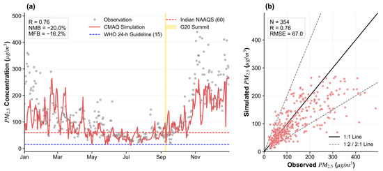
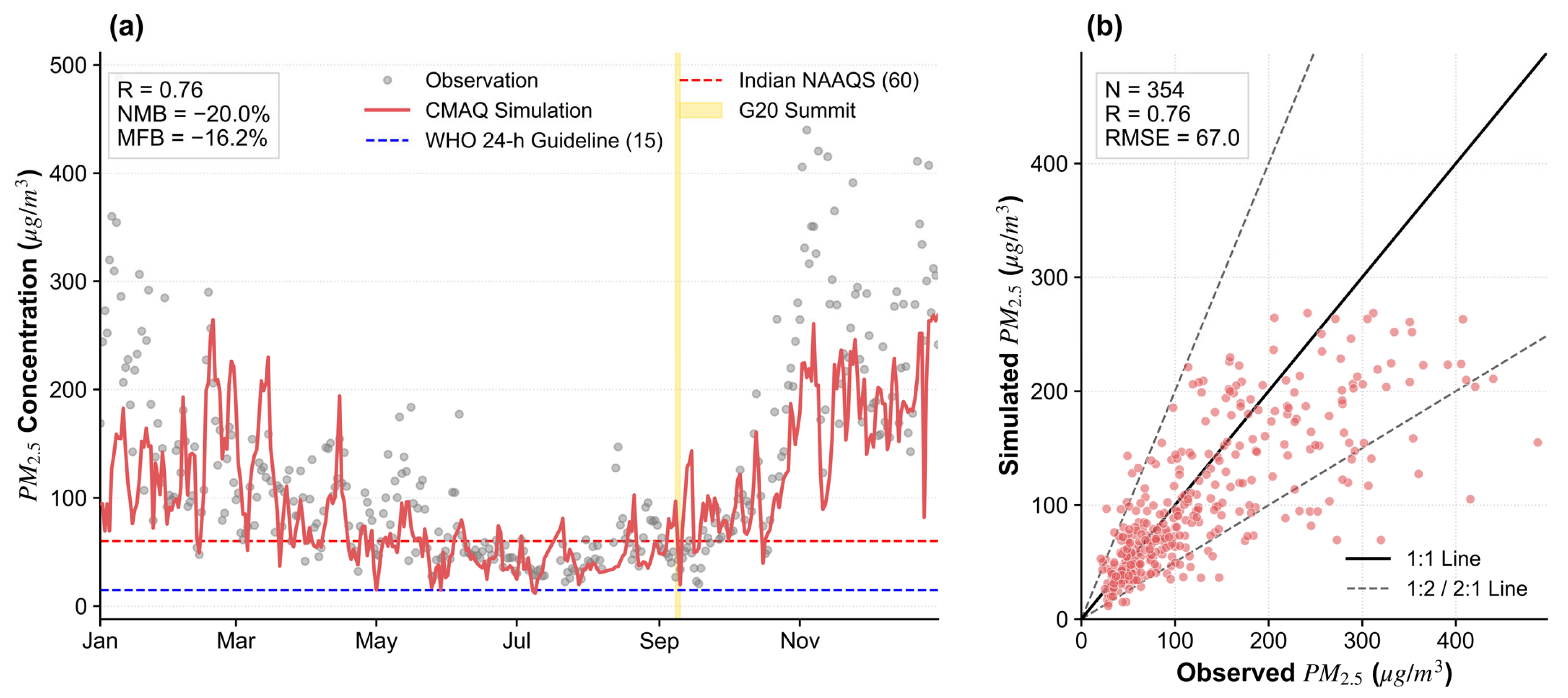
The model performance over New Delhi was also considered adequate for the purposes of this study. At the New Delhi scale, the observed and simulated annual mean PM2.5 concentrations in 2023 were 76.51 and 56.92 μg/m3, respectively, with an MFB of −0.26 and an MFE of 0.55 (Table 2). The negative MFB indicates an underestimation of PM2.5, which may be associated with uncertainties in local emissions and the smoothing of urban pollution hotspots at the 36 km model resolution. In addition to the New Delhi-scale statistical evaluation, Figure 2 further shows the daily PM2.5 variation at a representative monitoring site in New Delhi. As shown in Figure 2a, the model generally reproduced the seasonal cycle and day-to-day variability of PM2.5, including the elevated pollution levels during the post-monsoon period and the temporal fluctuations around the G20 summit. However, several high-concentration episodes exceeding 250 μg/m3 were underestimated, indicating that the model was less capable of capturing extreme daily peaks at the site scale [13,39]. Such site-level PM2.5 extremes in New Delhi can be strongly influenced by highly localized emissions and short-term accumulation processes, which are difficult to fully resolve at the 36 km model resolution. The scatter plot in Figure 2b shows a reasonable correlation coefficient (r) of 0.76, and most data points fall within the 1:2 and 2:1 dashed lines, suggesting that the model reasonably reproduced the general magnitude of PM2.5 despite the underestimation of some high-concentration episodes. For O3, the observed and simulated annual mean concentrations at the New Delhi scale were 71.69 and 78.57 ppb, respectively, with an MFB of 0.12 and an MFE of 0.39. The higher uncertainty in O3 modeling compared to PM2.5 is a documented challenge in South Asian studies, often attributed to complex emission structures and sharp meteorological fluctuations during the monsoon-withdrawal period [13,25]. Despite this uncertainty, the simulation generally captured the seasonal cycle and peak timing of O3 over Delhi.
Figure 2.
Evaluation of simulated daily PM2.5 concentrations at a representative monitoring site in New Delhi in 2023. (a) Time series of observed and simulated daily PM2.5 concentrations in New Delhi throughout 2023. Gray dots represent ground-based observations from the CPCB network, and the red solid line represents WRF-CMAQ simulation results. The blue and red dashed lines denote the WHO 24 h air quality guideline (15 μg/m3) and the Indian National Ambient Air Quality Standards (NAAQS, 60 μg/m3), respectively. The yellow shaded area highlights the G20 Summit period (September 8–10, 2023). Statistical metrics, including the correlation coefficient (r), normalized mean bias (NMB), and mean fractional bias (MFB), are provided in the inset. (b) Scatter plot of observed versus simulated daily PM2.5 concentrations. The solid black line indicates the 1:1 ratio, while the dashed lines represent the 1:2 and 2:1 boundaries, indicating factor-of-two performance (FAC2). Statistical metrics, including the number of samples (N), correlation coefficient (r), and root-mean-square error (RMSE), are shown in the inset. Each point represents a daily mean concentration.
Overall, the evaluation results suggest that the model provides a reasonable basis for analyzing the temporal evolution and scenario-based changes in PM2.5 and O3 during the G20 period. Although the model did not fully reproduce individual extreme PM2.5 peaks at the representative site, the overall statistical performance indicates that it can reasonably represent the general pollution level and temporal variability relevant to this study. Since the primary objective of this work is to investigate stage-dependent responses and quantify the relative impacts of meteorology and short-term emission controls, rather than to predict individual extreme daily concentrations, the current model performance is considered adequate for the subsequent attribution analysis.
3.2. Evolution of PM2.5 and O3 During the G20 Period
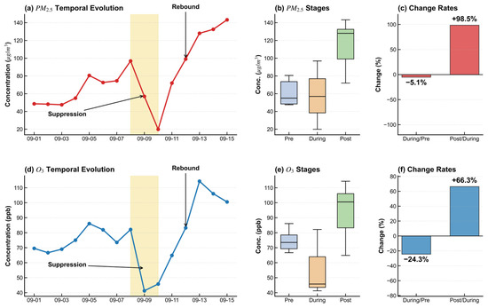
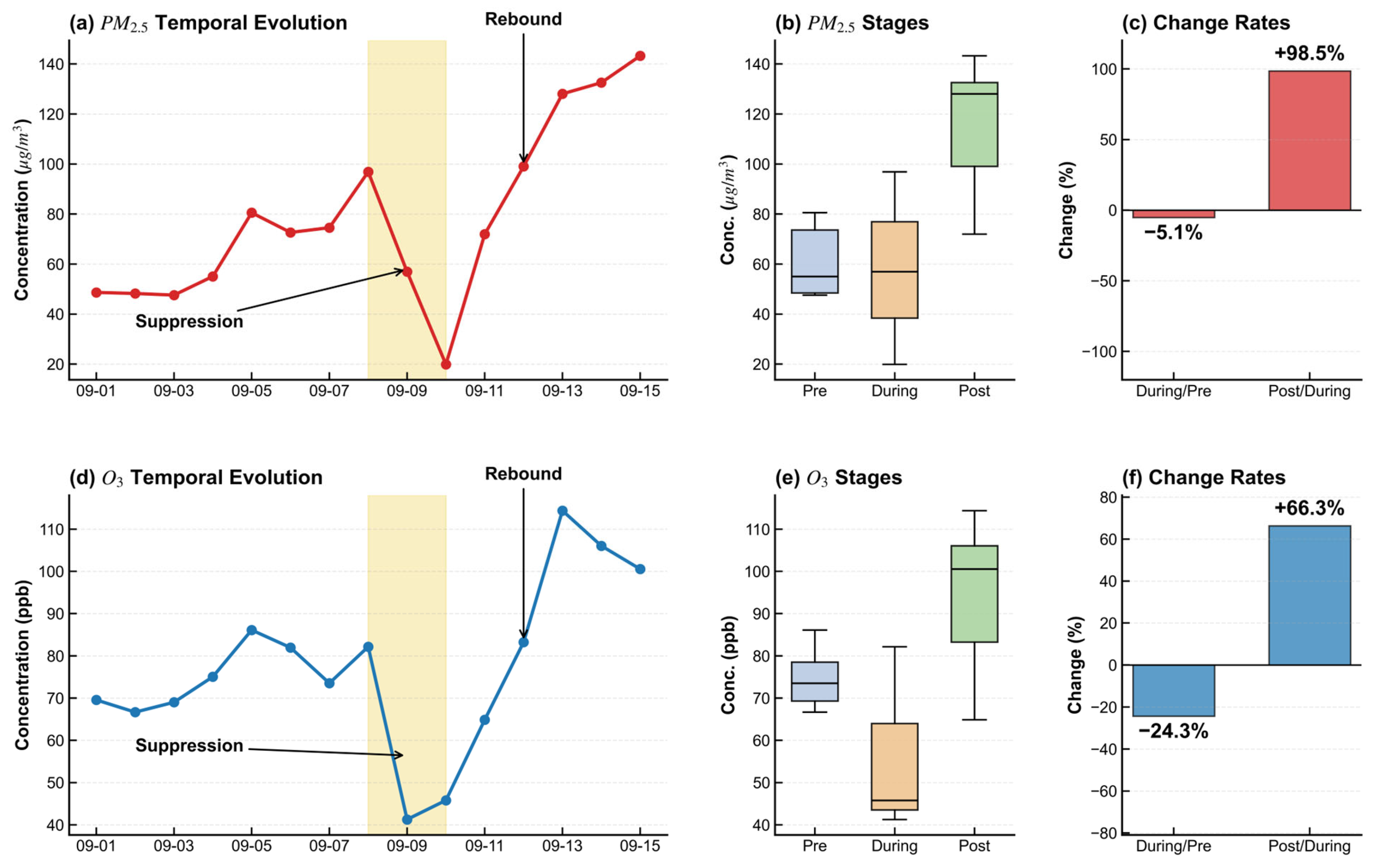
To characterize the evolution of air pollution during the 2023 G20 Summit, the period from 1 to 15 September 2023 was divided into three stages based on the S2 simulation: pre-G20 (1–7 September), during-G20 (8–10 September), and post-G20 (11–15 September). Both PM2.5 and O3 exhibited pronounced stage-dependent variations over New Delhi, as illustrated in Figure 3.
Figure 3.
Evolution of PM2.5 and MDA8 O3 concentrations in New Delhi during the G20 Summit period (1–15 September 2023). (a) Temporal variation in daily mean concentrations, where the yellow shaded area denotes the summit period (8–10 September). (b) Box-plots of concentration distributions across the pre-G20, during-G20, and post-G20 stages. (c) Percentage changes in mean concentrations between successive stages. (d) Temporal variation in MDA8 O3 concentrations. (e) Box plots of MDA8 O3 concentrations for the three stages. (f) Percentage changes in mean MDA8 O3 concentrations between successive stages.
As shown in Figure 3a, PM2.5 generally followed a pattern of pre-event accumulation, short-term alleviation during the summit, and rapid rebound afterward. The mean PM2.5 concentration was 61.04 μg/m3 during the pre-G20 stage and decreased slightly to 57.91 μg/m3 during the summit, indicating that the accumulation trend was partly suppressed. This 5.13% reduction (Figure 3c) indicates that the rising accumulation trend was effectively interrupted by the short-term administrative controls. However, PM2.5 increased sharply after the summit, with a stage mean of 114.96 μg/m3—a remarkable 98.52% increase relative to the summit period. The boxplot in Figure 3b further shows that post-G20 PM2.5 was characterized not only by higher mean and median values, but also by a persistently elevated lower bound, suggesting a more continuous and accumulated pollution episode after the event.
A similar stage-dependent pattern was also found for O3 (Figure 3d). The mean MDA8 O3 concentration was 74.56 ppb during the pre-G20 stage, decreased to 56.41 ppb during the summit, and then rose rapidly to 93.82 ppb in the post-G20 stage. Compared with PM2.5, O3 showed a stronger decline during the summit, with a reduction of 24.34% relative to the pre-G20 level (Figure 3f). This suggests that O3 was more sensitive to short-term changes in emissions and meteorological conditions during the event. After the summit, both pollutants rebounded markedly, but PM2.5 showed a stronger relative increase (98.52%) than O3 (66.32%), suggesting that pollutant concentrations rebounded rapidly after the summit under the evolving late-monsoon background.
The spatial difference maps further reveal distinct but coherent regional responses for the two pollutants. As shown in Figure S1a,b, PM2.5 changes during the summit relative to the pre-G20 stage were spatially heterogeneous, with negative differences mainly over the eastern and southeastern parts of the study region, while some western areas still showed positive anomalies. In contrast, the post-G20 period exhibited widespread positive differences across nearly the entire region, indicating a pronounced regional rebound of PM2.5. O3 showed a more spatially coherent response (Figure S1c,d). During the summit, negative anomalies dominated almost the entire New Delhi region and its surroundings, suggesting a regional-scale decline in O3 rather than a purely urban-core response. After the summit, O3 increased again over almost all areas. Overall, PM2.5 and O3 both exhibited a clear ‘high before the summit, lower during the summit, and rebound afterward’ pattern, indicating a coordinated response of complex air pollution to the combined effects of short-term controls and changing meteorological conditions. However, the stronger reduction in O3 during the summit and the greater post-event rebound in PM2.5 also suggest that the two pollutants differed in sensitivity and underlying response mechanisms.
The stage-dependent pattern shown in Figure 3 is therefore not interpreted as the main novelty of this study. Rather, it provides the observational and diagnostic basis for the subsequent scenario-based attribution. The key objective is to quantify how much of the pollution enhancement was attributable to unfavorable meteorology, how much could be offset by graded emission controls, and whether PM2.5 and O3 responded differently to the same control framework.
3.3. Meteorological Penalty During the Monsoon Withdrawal Period
To isolate the effect of meteorological conditions during the G20 period, the S3 scenario was designed by keeping the 2023 emission levels identical to those in S2 while replacing the meteorological fields with those of September 2022. Under this framework, the difference between S2 and S3 can be primarily interpreted as the contribution of meteorological variability. This comparison is particularly relevant because September in northern India corresponds to the monsoon withdrawal period, during which rainfall weakens, wet scavenging decreases, and atmospheric dispersion conditions gradually shift from relatively favorable monsoon conditions to a more stagnant environment that promotes pollution accumulation [12,39].
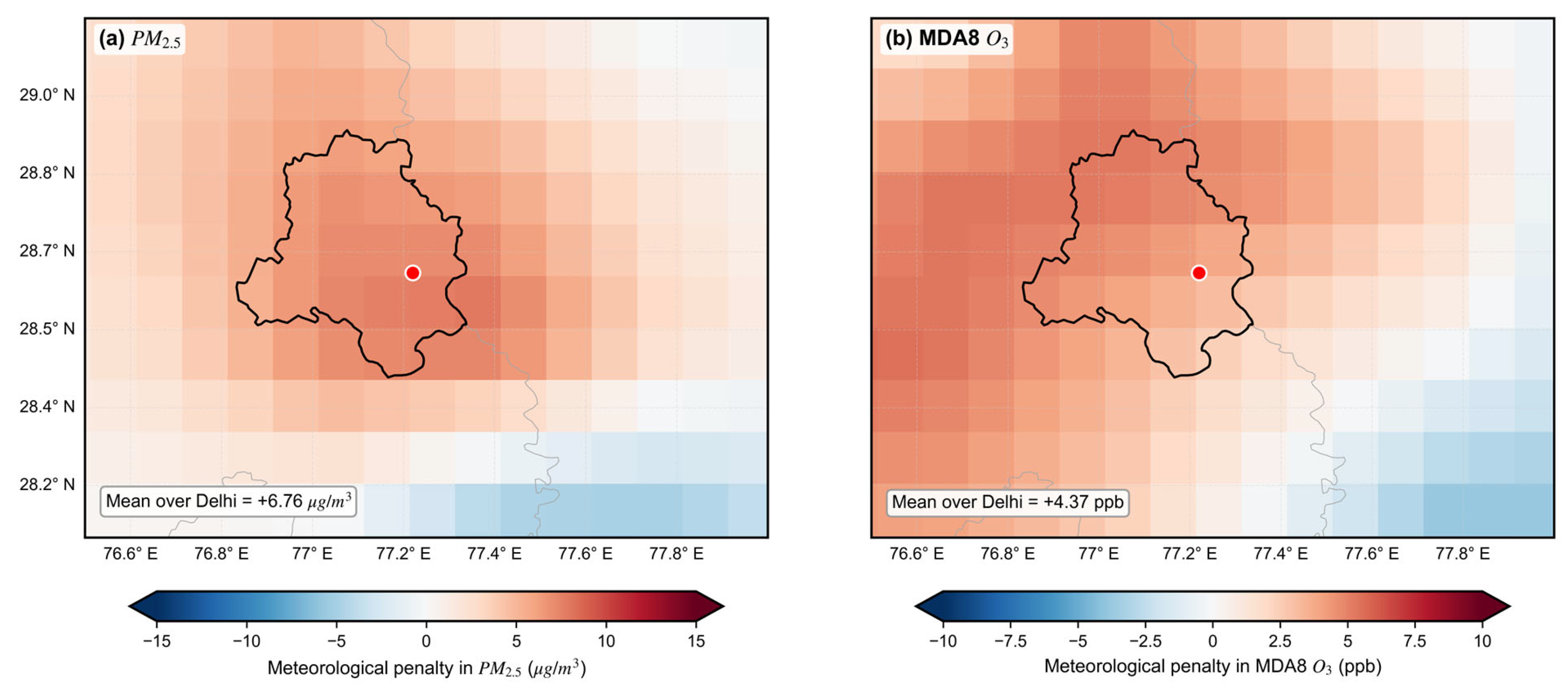
The comparison between S2 and S3 indicates a clear meteorological penalty in September 2023 over New Delhi. Under identical emissions, the PM2.5 concentration in New Delhi increased from 72.25 μg/m3 in S3 to 79.01 μg/m3 in S2, corresponding to a meteorology-driven increment of 6.76 μg/m3. For O3, the concentration increased from 76.82 ppb in S3 to 81.19 ppb in S2, yielding an increment of 4.37 ppb. These results show that the 2023 meteorological background amplified both particulate and ozone pollution, with a stronger effect on PM2.5 than on O3. The larger sensitivity of PM2.5 suggests that the unfavorable meteorological conditions during the monsoon withdrawal period were particularly effective in enhancing particle accumulation through reduced dispersion and weaker removal processes [12,40].
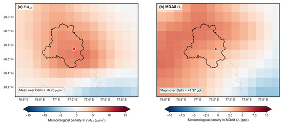
The spatial distributions further support this conclusion. As shown in Figure 4, the S2 and S3 differences were predominantly positive over New Delhi and its surrounding areas for both PM2.5 and O3, indicating that the meteorological penalty was not confined to the urban core but occurred at the regional scale. Therefore, the air quality changes during the G20 period did not take place under a neutral meteorological background. Instead, the summit was held under conditions that inherently favored pollution build-up. This result is important for the subsequent control-efficiency analysis, because any reduction achieved under the S4 scenarios should be interpreted as mitigation realized under an unfavorable meteorological background rather than under naturally improved atmospheric conditions.
Figure 4.
Spatial distribution of the quantified meteorological penalty for (a) PM2.5 (μg/m3) and (b) MDA8 O3 (ppb) across New Delhi and its surrounding regions. The penalty is defined as the difference between the S2 simulation (2023 meteorology) and the S3 simulation (2022 meteorology) under the same 2023 emission levels. Positive values (red) indicate that the 2023 meteorological conditions aggravated pollution, whereas negative values (blue) indicate a relative alleviation. The bold black outline denotes the administrative boundary of New Delhi, and the red dot marks the city center.
On the basis of this quantified meteorological penalty, the effectiveness of the graded emission-control scenarios was further evaluated to determine whether the short-term interventions could offset the unfavorable atmospheric background.
3.4. Response of PM2.5 and O3 to Graded Emission Control Scenarios
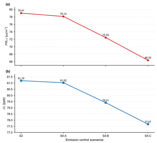
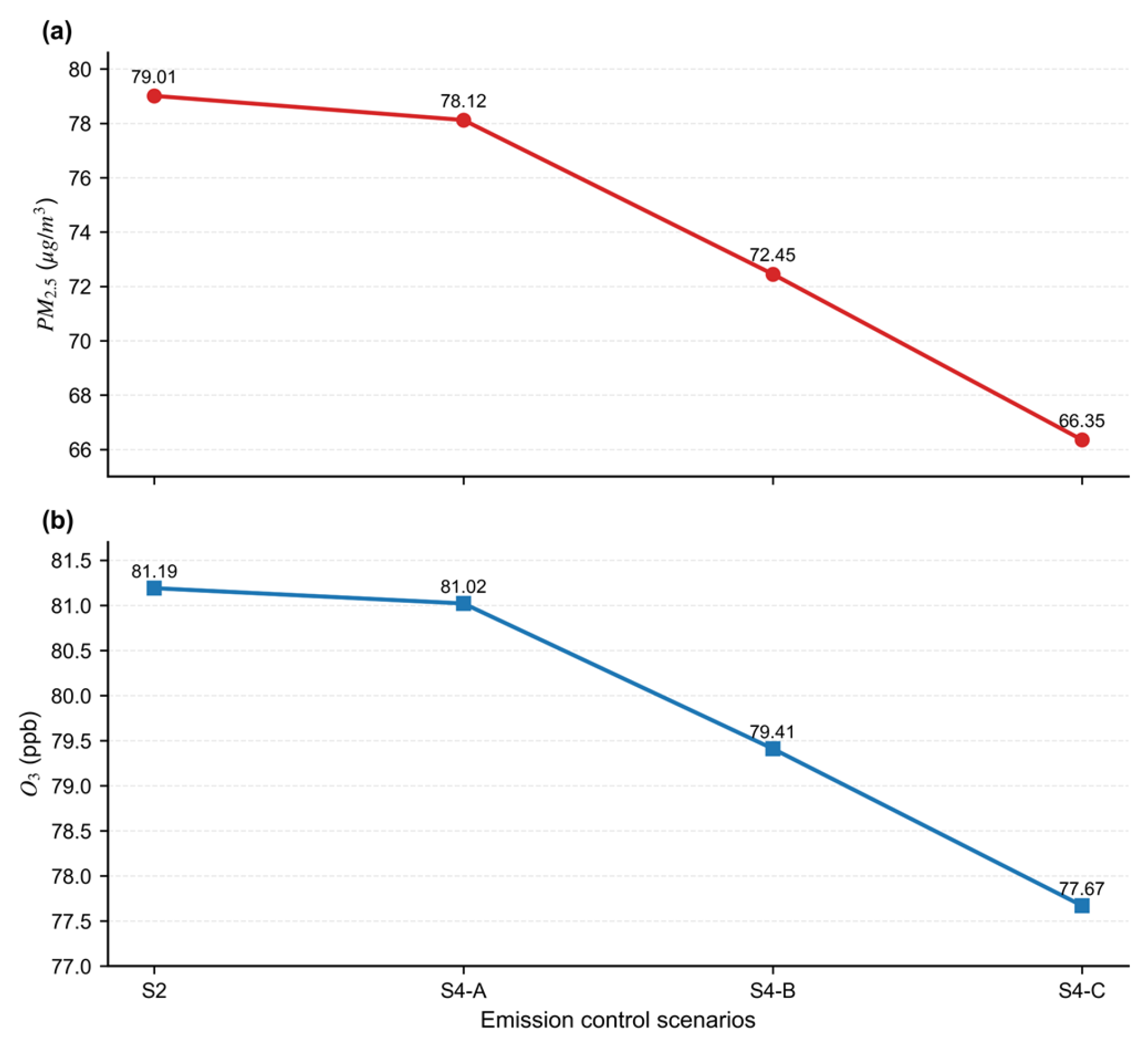
To evaluate the effectiveness of short-term administrative controls during the G20 period, the baseline scenario S2 was compared with the three graded control scenarios S4-A, S4-B, and S4-C, which represent progressively strengthened emission reductions. Figure 5 shows the concentration response of PM2.5 and MDA8 O3 under the four scenarios over New Delhi, while Figure S2 further illustrates the spatial differences in PM2.5 between each control scenario and S2. Together, these results provide a quantitative basis for assessing how air quality responded to increasing control intensity under the unfavorable meteorological background described above.
Figure 5.
Responses of (a) PM2.5 and (b) O3 concentrations in New Delhi under graded emission-control scenarios during the 2023 G20 period. S2 denotes the 2023 baseline scenario, while S4-A, S4-B, and S4-C represent progressively strengthened short-term control scenarios. PM2.5 and O3 both decreased as control intensity increased, with a more pronounced response emerging from S4-B onward.
PM2.5 showed a clear and progressive decline as the control intensity increased from S4-A to S4-C. Under the baseline scenario S2, the mean PM2.5 concentration in New Delhi was 79.01 μg/m3. This value decreased slightly to 78.12 μg/m3 under S4-A, indicating that the initial level of control only weakly suppressed particulate pollution. Under S4-B, PM2.5 decreased further to 72.45 μg/m3, showing a much stronger response than under S4-A. Under the most stringent scenario, S4-C, PM2.5 declined to 66.35 μg/m3, corresponding to the largest reduction among all scenarios. The spatial patterns of PM2.5 reduction were consistent with this concentration response. As shown in Figure S2, the negative PM2.5 anomalies relative to S2 were limited under S4-A, became more widespread under S4-B, and were strongest and most spatially coherent under S4-C, indicating that the effectiveness of emission controls increased not only in magnitude but also in regional extent.
O3 also decreased with increasing control intensity, although its response was weaker than that of PM2.5. The mean MDA8 O3 concentration was 81.19 ppb in S2, 81.02 ppb in S4-A, 79.41 ppb in S4-B, and 77.67 ppb in S4-C. The limited change from S2 to S4-A suggests that weak controls had only a minor influence on O3. In contrast, a clearer decline emerged under S4-B and became more pronounced under S4-C. Importantly, no obvious ozone rebound was found under any of the graded control scenarios. Instead, O3 decreased consistently as the controls were intensified, implying that the multisectoral reduction framework adopted in this study did not trigger a substantial unfavorable nonlinear ozone response over New Delhi [41]. To further examine this response, the HCHO/NO2 ratio was used as an indicator of the O3 chemical sensitivity regime over the 3 × 3 grid cells surrounding New Delhi. The ratios were 0.37, 0.38, 0.41, and 0.46 for S2, S4-A, S4-B, and S4-C, respectively (Table S4), all of which were below 1 and therefore indicated a VOC-limited regime [33]. Although the ratios increased slightly as the controls were strengthened, they remained within the same sensitivity regime, suggesting that the graded controls did not induce a major shift in O3 chemical sensitivity.
Taken together, the graded control scenarios reveal a distinct “stronger controls–lower concentrations” relationship for both pollutants, with PM2.5 responding more strongly than O3. The environmental benefit did not increase uniformly with control intensity. Rather, the response became markedly stronger after S4-B, suggesting that the inclusion and strengthening of additional source controls substantially enhanced the overall reduction efficiency. This pattern indicates that low-intensity or partially targeted controls were insufficient to produce substantial air-quality improvements during the summit period, whereas stronger and broader multisectoral controls were more effective in reducing both PM2.5 and O3 under adverse meteorological conditions.
3.5. PM2.5 Component Response to Coordinated Emission Controls
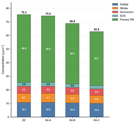
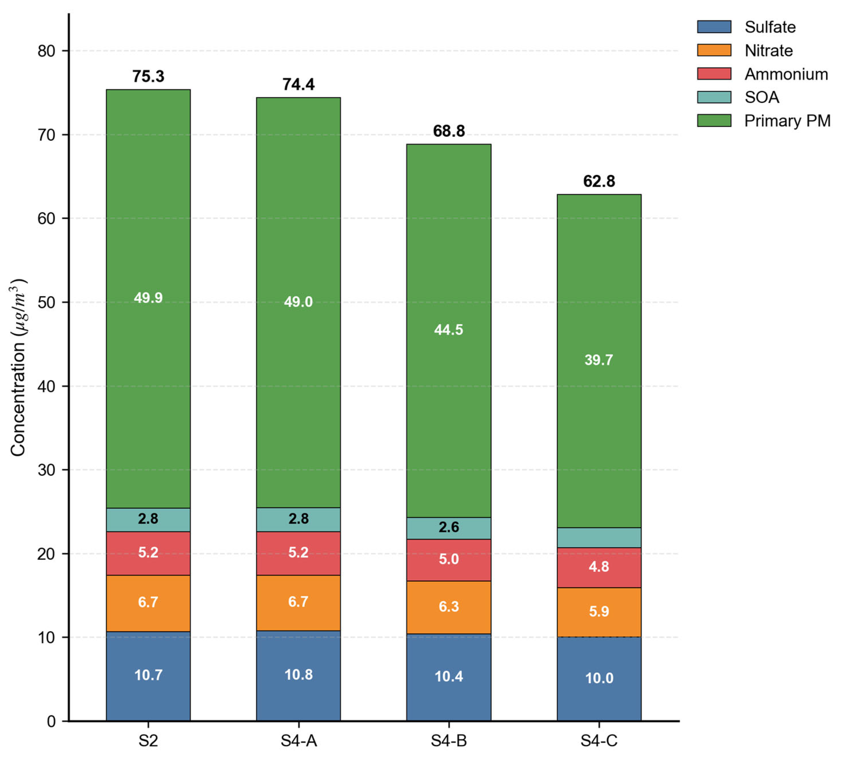
To further understand why PM2.5 responded more strongly than O3 under the graded control scenarios, the relative changes in major PM2.5 components were examined for S2, S4-A, S4-B, and S4-C (Figure 6). Because component-level observations were not available for direct validation, this analysis focuses on the relative response of simulated PM2.5 components among scenarios rather than on the absolute accuracy of individual component concentrations. Overall, the total concentration represented by the summed major PM2.5 components decreased progressively as the control intensity increased, indicating that multisectoral emission reductions not only lowered the bulk PM2.5 level but also systematically altered its chemical composition. The summed concentration of the major components decreased from 75.34 μg/m3 in S2 to 74.38 μg/m3 in S4-A, 68.81 μg/m3 in S4-B, and 62.83 μg/m3 in S4-C, corresponding to a total reduction of 12.51 μg/m3 under the most stringent control scenario.
Figure 6.
Major PM2.5 component responses under graded emission control scenarios over New Delhi in September 2023. Stacked bars show the monthly mean concentrations of sulfate, nitrate, ammonium, SOA, and primary PM for S2, S4-A, S4-B, and S4-C. Primary PM denotes the directly emitted primary aerosol fraction represented in the COMBINE output, calculated as EC + OC, where EC and OC denote elemental carbon and organic carbon, respectively. It excludes secondary components such as sulfate, nitrate, ammonium, and SOA. Numbers within the bars indicate individual component concentrations, and numbers above the bars indicate the sum of the selected components.
Primary particulate matter (Primary PM) was the dominant contributor to the PM2.5 reduction. Its concentration decreased from 49.93 μg/m3 in S2 to 39.75 μg/m3 in S4-C, yielding an absolute reduction of 10.18 μg/m3, which accounted for the majority of the total decrease in PM2.5 components. In addition, the fractional contribution of Primary PM to total PM2.5 decreased from 66.27% in S2 to 63.27% in S4-C. These results indicate that the short-term control measures were particularly effective in reducing primary particle emissions associated with road traffic, construction and road dust, and industrial direct emissions. Therefore, the rapid decline in Primary PM constitutes the main pathway through which the graded controls improved particulate air quality during the summit period.
Secondary components also showed coherent but weaker declines. Nitrate decreased from 6.73 μg/m3 in S2 to 5.90 μg/m3 in S4-C, corresponding to a reduction of 0.83 μg/m3. Sulfate, ammonium, and SOA also declined to varying extents under stronger control scenarios. Although the magnitude of these reductions was smaller than that of Primary PM, their consistent downward trends suggest that the coordinated controls affected not only direct particle emissions but also the formation of secondary aerosols. In particular, the decrease in nitrate implies that reductions in precursor emissions from traffic and industrial sources likely suppressed part of the secondary inorganic aerosol production during the control period.
The component changes also reveal a non-uniform response across scenarios. The improvement from S4-A to S4-B was much larger than that from S2 to S4-A, indicating that the control benefit did not increase linearly with the nominal control intensity. Instead, the response became markedly stronger once the broader multisector control structure was introduced and strengthened. This enhanced response was also related to the spatial distribution of the controlled emission sectors, as the on-road, construction/road-dust, and industrial sources showed distinct spatial patterns over New Delhi and its surrounding region (Figure S3). The inclusion of industrial point-source controls from S4-B onward likely expanded the effective spatial influence of emission reductions, contributing to the stronger decline in both primary and secondary PM2.5 components. This pattern suggests that while traffic and dust controls provided the initial reduction in Primary PM, the inclusion of additional source controls enhanced both the direct reduction in primary particles and the suppression of secondary formation. As a result, the coordinated short-term control strategy produced a structurally consistent decline in both primary and secondary PM2.5 components, thereby explaining the pronounced response of total PM2.5 under the stronger scenarios.
3.6. Spatial Benefits of Deep Emission Reduction and Co-Control Implications
Among all control scenarios, S4-C represents the most stringent and comprehensive emission-reduction strategy, and it produced the largest improvements in both PM2.5 and O3. To further assess its environmental benefit, the spatial differences between S4-C and the baseline scenario S2 were analyzed, with a focus on whether deep short-term controls could simultaneously mitigate particulate and ozone pollution under the unfavorable meteorological background during the G20 period.
For PM2.5, the S4-C scenario produced widespread negative anomalies over New Delhi and its surrounding region (Figure S4a), indicating that deep emission reduction lowered particulate pollution not only in the urban core but also across the broader regional environment. Consistent with the concentration statistics presented above, the mean PM2.5 concentration in New Delhi decreased from 79.01 μg/m3 under S2 to 66.35 μg/m3 under S4-C, corresponding to an absolute reduction of 12.66 μg/m3. The spatially coherent decrease suggests that the combined controls on traffic, construction, and road dust, and industrial sources were capable of suppressing PM2.5 accumulation at the regional scale, rather than producing only isolated local improvements.
A similarly favorable response was found for O3. The mean MDA8 O3 concentration decreased from 81.19 ppb in S2 to 77.67 ppb in S4-C, corresponding to a reduction of 3.52 ppb. As shown in Figure S4b, the S4-C–S2 differences were predominantly negative over New Delhi and its surrounding areas, suggesting that the strengthened multisectoral control strategy did not induce an obvious ozone rebound. Instead, O3 generally declined under S4-C, indicating that the coordinated reduction in precursor emissions in this study exerted a net positive effect on ozone control. This result is particularly important because it implies that the deep control scenario was able to improve both PM2.5 and O3 simultaneously, rather than shifting the burden from one pollutant to the other.
The comparison between meteorological penalty and control benefit further highlights the significance of S4-C (Figure S5). For PM2.5, the unfavorable meteorological conditions in September 2023 increased the concentration by 6.76 μg/m3, whereas the S4-C control reduced it by 12.66 μg/m3, resulting in a net decrease of 5.90 μg/m3 relative to the 2022-meteorology reference state. For O3, the meteorological penalty was 4.37 ppb, while the S4-C control benefit was 3.52 ppb, indicating that the control measures substantially suppressed the ozone enhancement but did not fully offset the adverse meteorological effect. Taken together, these results show that deep coordinated emission controls were sufficient to overcome the unfavorable meteorological background for PM2.5, and were also effective in mitigating, though not fully neutralizing, the meteorological penalty for O3. Therefore, under complex late-monsoon conditions, high-intensity multisectoral controls provide a more effective pathway for PM2.5–O3 co-control than weaker or more limited interventions.
4. Discussion
4.1. Role of Adverse Meteorology During the Monsoon Withdrawal Period
The results indicate that the 2023 G20 Summit took place under a distinctly unfavorable meteorological background rather than under naturally improved atmospheric conditions. During the monsoon withdrawal period, rainfall weakens, wet scavenging becomes less effective, and atmospheric dispersion gradually shifts from relatively favorable monsoon conditions to a more stagnant environment. Under such a background, pollutants are more likely to accumulate over New Delhi and its surrounding region. This helps explain why both PM2.5 and O3 were higher in S2 than in S3, despite identical emissions in the two scenarios. This interpretation is consistent with previous studies showing that post-monsoon pollution over northern India is strongly amplified by stagnant meteorological conditions, weakened wet scavenging, and reduced boundary-layer ventilation [11,39,42].
The stronger meteorological penalty for PM2.5 than for O3 suggests that particulate pollution was more directly affected by the deterioration of dispersion and removal conditions. Reduced boundary-layer ventilation and weaker wet deposition can rapidly enhance PM2.5 accumulation, especially during the transitional period from the monsoon season to the autumn pollution season. In contrast, O3 was also elevated under the 2023 meteorological background, but its increase was smaller, implying that ozone was influenced by both meteorological enhancement and chemical constraints. Therefore, the summit-period pollution control should be interpreted as mitigation achieved under a meteorologically unfavorable regime, which makes the subsequent control benefits more meaningful. The stronger sensitivity of PM2.5 than O3 also agrees with earlier findings that particulate accumulation over India is more directly enhanced by stagnant conditions, whereas ozone reflects a combined influence of meteorological forcing and chemical constraints [5].
4.2. Different Sensitivities of PM2.5 and O3 to Short-Term Coordinated Controls
A major finding of this study is that PM2.5 responded more strongly than O3 to the graded short-term control scenarios. This difference is physically plausible because PM2.5 during the study period was dominated by primary particulate matter, which can be reduced directly and rapidly through restrictions on traffic, construction activities, road dust, and industrial emissions. The component analysis showed that Primary PM accounted for most of the PM2.5 reduction under S4-C, indicating that short-term administrative controls were highly effective in suppressing direct particle emissions.
By contrast, O3 showed a weaker but still consistently negative response. This suggests that ozone during the G20 period was influenced by a more complex combination of precursor emissions, chemical sensitivity, and meteorological conditions. The HCHO/NO2 diagnostic further indicated a VOC-limited regime over the New Delhi control region across all scenarios (Table S4). This result suggests that isolated NOx reductions could potentially enhance O3 through weakened titration, especially under VOC-limited conditions [33,43]. However, the present control scenarios were not NOx-only cases; instead, they represented coordinated multisectoral reductions that likely affected multiple precursor streams simultaneously. Therefore, the absence of a strong O3 rebound under S4-A/B/C is consistent with the interpretation that broader coordinated controls can provide co-benefits for PM2.5 and O3 rather than triggering an unfavorable nonlinear ozone response [8,44]. Nevertheless, the S4-C control benefit for O3 did not fully offset the meteorological penalty, indicating that ozone remained more sensitive than PM2.5 to the combined influence of background meteorology and precursor chemistry.
4.3. Strengthened Reduction Benefits After S4-B
The control benefits did not increase uniformly with nominal control intensity. Instead, both PM2.5 and O3 showed a much stronger response after S4-B than after S4-A. This pattern suggests that the environmental effectiveness of short-term controls depended not only on the magnitude of emission reduction, but also on the breadth of the source sectors included in the control strategy. Under S4-A, the controls mainly targeted traffic and dust-related sources, which produced only limited improvements in both PM2.5 and O3. Once broader source controls were incorporated and strengthened in S4-B and S4-C, the benefits became substantially larger.
The stronger response after S4-B may reflect the added importance of industrial-source control in the overall reduction framework. Industrial emissions can contribute both directly to primary particulate matter and indirectly to secondary aerosol formation through precursor emissions such as NOx and SO2 [45,46]. Therefore, the enhanced benefits under S4-B and S4-C likely arose from a combination of direct suppression of primary PM and partial inhibition of secondary particle formation. Nevertheless, this interpretation should be treated cautiously. Because S4-A, S4-B, and S4-C are cumulative control scenarios rather than single-source sensitivity experiments, the present results support an inference about enhanced marginal benefit rather than a strict attribution of nonlinear effects to one specific source category.
This pattern is also consistent with previous event-based studies showing that narrowly targeted measures, such as traffic-only restrictions, often yield limited air-quality improvements, whereas broader multi-sectoral interventions tend to produce substantially larger benefits [9,47,48]. This interpretation is further supported by recent studies suggesting that, under unfavorable meteorological conditions, multisectoral and regional-scale controls may provide substantially larger marginal benefits than localized single-sector measures [49]. The enhanced response after S4-B therefore likely reflects not only a stronger nominal reduction level, but also the greater effectiveness of broader coordinated controls under an adverse atmospheric background.
4.4. Implications for Co-Control and Study Limitations
The present results have direct implications for air-quality management during major events under complex meteorological conditions. First, low-intensity or narrowly targeted measures may be insufficient to achieve substantial air-quality improvements when the atmospheric background already favors pollution accumulation. Second, high-intensity multisectoral controls can provide meaningful co-benefits for PM2.5 and O3, particularly when they simultaneously reduce primary particulate emissions and gaseous precursors. This broader implication is consistent with previous studies emphasizing the importance of coordinated PM2.5–O3 control strategies rather than single-pollutant management, and with earlier sensitivity analyses over Delhi showing that broader coordinated precursor reductions are more likely to avoid unfavorable ozone responses than isolated controls [3,8]. For New Delhi during the G20 period, the deepest control scenario was able to overcome the meteorological penalty for PM2.5 and substantially mitigate the penalty for O3, highlighting the value of coordinated PM2.5–O3 control strategies rather than single-pollutant management. More broadly, the present findings are also in line with previous work indicating that air-pollution episodes in India are jointly shaped by complex source mixtures and unfavorable regional meteorology, especially during stagnant post-monsoon conditions [6,11]. They also agree with earlier studies showing that PM2.5 and O3 do not respond identically to changes in emissions and meteorology, with particulate pollution generally exhibiting a more direct sensitivity to accumulation conditions, whereas ozone remains constrained by more complex precursor chemistry [5]. Relative to these earlier studies, the present work further quantifies the competition between meteorological penalty and graded control benefit within a unified PM2.5–O3 co-control framework during a real major-event period.
Several limitations should also be acknowledged. First, the emission-reduction scenarios were idealized and based on prescribed scaling factors rather than near-real-time, observation-constrained short-term activity data for each source sector. This source of uncertainty is not unique to the present study, but reflects a broader challenge in India air-quality modeling, where timely sector-resolved inventories remain limited and emission updates often rely on proxy-based scaling approaches [14,15]. Although this strategy is commonly used when timely regional inventories are unavailable, it may not fully capture short-term fluctuations in actual emissions during the G20 period. Second, although the ozone sensitivity regime was diagnosed using the HCHO/NO2 ratio, the discussion of ozone response is primarily based on concentration changes and does not explicitly resolve the underlying radical chemistry or detailed ozone formation pathways. Third, uncertainty remains in the simulated PM2.5 chemical composition because continuous component-level observations were not available for direct validation. Although the total PM2.5 performance was evaluated against CPCB observations and was considered adequate for the scenario-based analysis, routine observations do not provide sufficient component-level data to directly validate simulated sulfate, nitrate, ammonium, SOA, and primary PM. As a result, the component analysis in this study should be interpreted mainly as a diagnostic assessment of relative changes among emission-control scenarios, rather than as a fully validated estimate of absolute component concentrations. Uncertainties in emission speciation, primary particle emissions, precursor emissions, and aerosol thermodynamic partitioning may lead to overestimation or underestimation of individual components, especially nitrate, ammonium, SOA, and primary PM [50,51]. Fourth, this analysis focuses on a single major event during one monsoon-withdrawal period, and the extent to which the findings can be generalized to other cities, seasons, or event types remains uncertain. Future work should therefore incorporate source-specific sensitivity experiments, improved short-term activity constraints, ground-based or campaign-based PM2.5 composition measurements, and broader event-based comparisons to better constrain the mechanisms and generalizability of coordinated emission-control effects.
5. Conclusions
This study quantified the relative roles of meteorology and graded short-term emission controls in shaping PM2.5 and ozone changes during the 2023 G20 Summit in New Delhi using the WRF-CMAQ modeling framework. Both pollutants exhibited clear stage-dependent variations, with lower concentrations during the summit and rapid rebound afterward. The comparison between S2 and S3 revealed a distinct meteorological penalty in September 2023, indicating that the summit took place under atmospheric conditions favorable for pollution accumulation rather than under naturally improved conditions. The penalty was stronger for PM2.5 than for MDA8 O3, highlighting the greater sensitivity of particulate pollution to reduced dispersion and weaker removal during the monsoon withdrawal period. Under the graded control scenarios, both PM2.5 and O3 decreased with increasing control intensity, and the strongest scenario, S4-C, produced the largest air-quality benefits. Component analysis further showed that the PM2.5 reduction was dominated by the decline in primary particulate matter, while secondary components also decreased consistently. Deep coordinated controls were sufficient to overcome the meteorological penalty for PM2.5 and substantially mitigate, though not fully offset, the penalty for O3. These findings highlight the importance of high-intensity multisectoral controls for PM2.5–O3 co-control during major events under unfavorable meteorological conditions. More broadly, the framework developed in this study can be extended to other megacities to assess whether emission-control intensity is sufficient to offset meteorological penalties under extreme atmospheric conditions.
Supplementary Materials
The following supporting information can be downloaded at: https://www.mdpi.com/article/10.3390/atmos17060584/s1, Table S1. Sector-specific scaling factors applied to update EDGAR v8.1 emissions from 2022 to 2023. Table S2. Model configuration. Table S3. Statistical performance of WRF-simulated meteorological variables over India in representative months of 2023. Table S4. HCHO/NO2 ratios over the 3 × 3 grid cells surrounding New Delhi in September 2023. Figure S1. Spatial distribution of differences in daily mean PM2.5 and MDA8 O3 concentrations over New Delhi and its surrounding regions during the G20 period. Figure S2. Spatial progression of changes in PM2.5 concentration over New Delhi and surrounding areas under graded emission control scenarios. Figure S3. Spatial distributions of September mean primary carbonaceous particulate emissions from controlled EDGAR sectors over New Delhi and surrounding regions. Figure S4. Spatial benefits of deep emission reduction for (a) PM2.5 and (b) MDA8 O3 over New Delhi and surrounding areas under the S4-C scenario. Figure S5. Comparison of unfavorable meteorological impacts and S4-C control benefits on changes in PM2.5 and MDA8 O3 over New Delhi.
Author Contributions
Conceptualization, Z.H. and H.Z.; methodology, Z.H. and H.Z.; software, Z.H.; validation, Z.H.; formal analysis, Z.H.; investigation, Z.H.; data curation, Z.H. and M.Z.; writing—original draft preparation, Z.H.; writing—review and editing, Z.H., C.T., M.Z., S.W., H.Z. and Y.C.; visualization, Z.H.; supervision, H.Z. and Y.C. All authors have read and agreed to the published version of the manuscript.
Funding
This research received no external funding.
Institutional Review Board Statement
Not applicable.
Informed Consent Statement
Not applicable.
Data Availability Statement
The observational and input datasets used in this study are publicly available from the corresponding official sources, including CPCB, EDGAR v8.1, MEGAN v2.1, FINN v2.5, and NCEP FNL. The model output data and processed datasets generated in this study are available from the corresponding author upon reasonable request.
Acknowledgments
AI-assisted tools were used for language editing during the preparation of this manuscript. The authors reviewed and edited all outputs and take full responsibility for the content of this publication. The authors thank their colleagues and research group members for constructive discussions and technical support during this study.
Conflicts of Interest
The authors declare no conflicts of interest.
Abbreviations
The following abbreviations are used in this manuscript:
| AERO6 | Sixth-generation CMAQ aerosol module |
| CMAQ | Community Multiscale Air Quality |
| CPCB | Central Pollution Control Board |
| EC | Elemental Carbon |
| EDGAR | Emissions Database for Global Atmospheric Research |
| FAC2 | Factor of Two |
| FINN | Fire Inventory from NCAR |
| FNL | Final Analysis |
| G20 | Group of Twenty |
| GE | Gross Error |
| HCHO | Formaldehyde |
| MB | Mean Bias |
| MDA8 | Maximum Daily 8 h Average |
| MEGAN | Model of Emissions of Gases and Aerosols from Nature |
| MFB | Mean Fractional Bias |
| MFE | Mean Fractional Error |
| NAAQS | National Ambient Air Quality Standards |
| NCEP | National Centers for Environmental Prediction |
| NH3 | Ammonia |
| NMB | Normalized Mean Bias |
| NO2 | Nitrogen dioxide |
| NOx | Nitrogen oxides |
| O3 | Ozone |
| OBS | Observed mean concentration |
| OC | Organic Carbon |
| PBL | Planetary Boundary Layer |
| PEC | Particulate elemental carbon |
| PM2.5 | Fine particulate matter with aerodynamic diameter ≤ 2.5 μm |
| PNO3 | Particulate nitrate |
| POC | Particulate organic carbon |
| PRE | Predicted mean concentration |
| PSO4 | Particulate sulfate |
| R | Correlation coefficient |
| RH | Relative Humidity |
| RMSE | Root Mean Square Error |
| SAPRC-11 | Statewide Air Pollution Research Center 2011 mechanism |
| SNA | Sulfate–nitrate–ammonium |
| SO2 | Sulfur dioxide |
| SOA | Secondary Organic Aerosol |
| T2 | 2 m temperature |
| VOCs | Volatile Organic Compounds |
| WD | Wind Direction |
| WHO | World Health Organization |
| WRF | Weather Research and Forecasting |
| WS | 10 m Wind Speed |
References
- Lal, R.M.; Nagpure, A.S. Evaluation of India’s National Clean Air Program Performance and Potential Health Benefits. Environ. Sci. Technol. Lett. 2026. [Google Scholar] [CrossRef]
- Pandey, A.; Brauer, M.; Cropper, M.L.; Balakrishnan, K.; Mathur, P.; Dey, S.; Turkgulu, B.; Kumar, G.A.; Khare, M.; Beig, G.; et al. Health and Economic Impact of Air Pollution in the States of India: The Global Burden of Disease Study 2019. Lancet Planet. Health 2021, 5, e25–e38. [Google Scholar] [CrossRef] [PubMed]
- He, C.; Liu, J.; Zhou, Y.; Zhou, J.; Zhang, L.; Wang, Y.; Liu, L.; Peng, S. Synergistic PM2.5 and O3 Control to Address the Emerging Global PM2.5-O3 Compound Pollution Challenges. Eco-Environ. Health 2024, 3, 325–337. [Google Scholar] [CrossRef] [PubMed]
- Kumari, S.; Verma, N.; Lakhani, A.; Kumari, K.M. Severe Haze Events in the Indo-Gangetic Plain during Post-Monsoon: Synergetic Effect of Synoptic Meteorology and Crop Residue Burning Emission. Sci. Total Environ. 2021, 768, 145479. [Google Scholar] [CrossRef]
- Krishnaveni, A.S.; Madhavan, B.L.; Jain, C.D.; Venkat Ratnam, M. Spatial, Temporal Features and Influence of Meteorology on PM2.5 and O3 Association across Urban and Rural Environments of India. Atmos. Environ. X 2024, 22, 100265. [Google Scholar] [CrossRef]
- Venkataraman, C.; Anand, A.; Maji, S.; Barman, N.; Tiwari, D.; Muduchuru, K.; Sharma, A.; Gupta, G.; Bhardwaj, A.; Haswani, D.; et al. Drivers of PM2.5 Episodes and Exceedance in India: A Synthesis From the COALESCE Network. J. Geophys. Res. Atmos. 2024, 129, e2024JD040834. [Google Scholar] [CrossRef]
- Express News Service. In Bid to Control Air Quality for G20 Summit in Delhi, Govt to Deploy 30 Mobile Pollution Control Teams; The Indian Express: Noida, India, 2023; Available online: https://indianexpress.com/article/cities/delhi/delhi-pollution-control-committee-g20-summit-30-teams-lg-saxena-8878963/ (accessed on 1 June 2026).
- Chen, Y.; Wild, O.; Ryan, E.; Sahu, S.K.; Lowe, D.; Archer-Nicholls, S.; Wang, Y.; McFiggans, G.; Ansari, T.; Singh, V.; et al. Mitigation of PM2.5 and Ozone Pollution in Delhi: A Sensitivity Study during the Pre-Monsoon Period. Atmos. Chem. Phys. 2020, 20, 499–514. [Google Scholar] [CrossRef]
- Wang, P.; Dai, X.-G. “APEC Blue” Association with Emission Control and Meteorological Conditions Detected by Multi-Scale Statistics. Atmos. Res. 2016, 178–179, 497–505. [Google Scholar] [CrossRef]
- Ji, Y.; Qin, X.; Wang, B.; Xu, J.; Shen, J.; Chen, J.; Huang, K.; Deng, C.; Yan, R.; Xu, K.; et al. Counteractive Effects of Regional Transport and Emission Control on the Formation of Fine Particles: A Case Study during the Hangzhou G20 Summit. Atmos. Chem. Phys. 2018, 18, 13581–13600. [Google Scholar] [CrossRef]
- Zhou, M.; Xie, Y.; Wang, C.; Shen, L.; Mauzerall, D. Impacts of Current and Climate Induced Changes in Atmospheric Stagnation on Indian Surface PM2.5 Pollution. Nat. Commun. 2024, 15, 7448. [Google Scholar] [CrossRef]
- Beig, G.; Rathod, A.; Tikle, S.; Maji, S.; Sobhana, S.B. Association of Retreating Monsoon and Extreme Air Pollution in a Megacity. J. Environ. Sci. 2021, 106, 97–104. [Google Scholar] [CrossRef]
- Kota, S.H.; Guo, H.; Myllyvirta, L.; Hu, J.; Sahu, S.K.; Garaga, R.; Ying, Q.; Gao, A.; Dahiya, S.; Wang, Y.; et al. Year-Long Simulation of Gaseous and Particulate Air Pollutants in India. Atmos. Environ. 2018, 180, 244–255. [Google Scholar] [CrossRef]
- Zhou, M.; Mauzerall, D.L.; Velamuri, V.; Kota, S.H.; Nambiar, M.; Xie, Y. Surface PM2.5 Air Pollution in 2022 India: Emission Updates, WRF-Chem Model Evaluation, and Source Attribution. EGUsphere 2025. preprint. [Google Scholar] [CrossRef]
- Santra, S. PM2.5 in India: Spatiotemporal Trends, Source Contributions, and Health Impacts. Environ. Monit. Assess. 2025, 197, 1382. [Google Scholar] [CrossRef]
- Xiao, Q.; Zheng, Y.; Geng, G.; Chen, C.; Huang, X.; Che, H.; Zhang, X.; He, K.; Zhang, Q. Separating Emission and Meteorological Contributions to Long-Term PM2.5 Trends over Eastern China during 2000–2018. Atmos. Chem. Phys. 2021, 21, 9475–9496. [Google Scholar] [CrossRef]
- Mogno, C.; Palmer, P.I.; Marvin, M.R.; Sharma, S.; Chen, Y.; Wild, O. Road Transport Impact on PM2.5 Pollution over Delhi during the Post-Monsoon Season. Atmos. Environ. X 2023, 17, 100200. [Google Scholar] [CrossRef]
- Carter, W.P.L.; Heo, G. Development of Revised SAPRC Aromatics Mechanisms. Atmos. Environ. 2013, 77, 404–414. [Google Scholar] [CrossRef]
- Binkowski, F.S.; Roselle, S.J. Models-3 Community Multiscale Air Quality (CMAQ) Model Aerosol Component 1. Model Description. J. Geophys. Res. Atmos. 2003, 108, 4183. [Google Scholar] [CrossRef]
- Ying, Q.; Li, J.; Kota, S.H. Significant Contributions of Isoprene to Summertime Secondary Organic Aerosol in Eastern United States. Environ. Sci. Technol. 2015, 49, 7834–7842. [Google Scholar] [CrossRef]
- Crippa, M.; Guizzardi, D.; Pagani, F.; Schiavina, M.; Melchiorri, M.; Pisoni, E.; Graziosi, F.; Muntean, M.; Maes, J.; Dijkstra, L.; et al. Insights into the Spatial Distribution of Global, National, and Subnational Greenhouse Gas Emissions in the Emissions Database for Global Atmospheric Research (EDGAR v8.0). Earth Syst. Sci. Data 2024, 16, 2811–2830. [Google Scholar] [CrossRef]
- Wang, D.; Hu, J.; Xu, Y.; Lv, D.; Xie, X.; Kleeman, M.; Xing, J.; Zhang, H.; Ying, Q. Source Contributions to Primary and Secondary Inorganic Particulate Matter during a Severe Wintertime PM2.5 Pollution Episode in Xi’an, China. Atmos. Environ. 2014, 97, 182–194. [Google Scholar] [CrossRef]
- U.S. Environmental Protection Agency. SPECIATE 4.3: Addendum to SPECIATE 4.2 Speciation Database Development Documentation; U.S. Environmental Protection Agency: Washington, DC, USA, 2011.
- Wang, S.; Zhang, M.; Gao, Y.; Wang, P.; Fu, Q.; Zhang, H. Diagnosing Drivers of PM2.5 Simulation Biases in China from Meteorology, Chemical Composition, and Emission Sources Using an Efficient Machine Learning Method. Geosci. Model Dev. 2024, 17, 3617–3629. [Google Scholar] [CrossRef]
- Zhang, M.; Wang, S.; Han, Z.; Tao, C.; Wang, Y.; Kumar, M.N.; Dahiya, S.; Wang, P.; Zhang, H. Widening Cost-Benefits Gap of Emission Control Measures in India from 2017 to 2022. Atmos. Pollut. Res. 2025, 16, 102615. [Google Scholar] [CrossRef]
- Guenther, A.B.; Jiang, X.; Heald, C.L.; Sakulyanontvittaya, T.; Duhl, T.; Emmons, L.K.; Wang, X. The Model of Emissions of Gases and Aerosols from Nature Version 2.1 (MEGAN2.1): An Extended and Updated Framework for Modeling Biogenic Emissions. Geosci. Model Dev. 2012, 5, 1471–1492. [Google Scholar] [CrossRef]
- Thongsame, W.; Henze, D.K.; Kumar, R.; Barth, M.; Pfister, G. Evaluation of WRF-Chem PM2.5 Simulations in Thailand with Different Anthropogenic and Biomass-Burning Emissions. Atmos. Environ. X 2024, 23, 100282. [Google Scholar] [CrossRef]
- Wiedinmyer, C.; Kimura, Y.; McDonald-Buller, E.C.; Emmons, L.K.; Buchholz, R.R.; Tang, W.; Seto, K.; Joseph, M.B.; Barsanti, K.C.; Carlton, A.G.; et al. The Fire Inventory from NCAR Version 2.5: An Updated Global Fire Emissions Model for Climate and Chemistry Applications. Geosci. Model Dev. 2023, 16, 3873–3891. [Google Scholar] [CrossRef]
- Song, Y.; Lin, C.; Li, Y.; Lau, A.K.H.; Fung, J.C.H.; Lu, X.; Guo, C.; Ma, J.; Lao, X.Q. An Improved Decomposition Method to Differentiate Meteorological and Anthropogenic Effects on Air Pollution: A National Study in China during the COVID-19 Lockdown Period. Atmos. Environ. 2021, 250, 118270. [Google Scholar] [CrossRef]
- Zhang, H.; Tang, K.; Feng, W.; Yan, X.; Liao, H.; Li, N. Impact of Short-Term Emission Control Measures on Air Quality in Nanjing During the Jiangsu Development Summit. Front. Environ. Sci. 2021, 9, 693513. [Google Scholar] [CrossRef]
- Boylan, J.W.; Russell, A.G. PM and Light Extinction Model Performance Metrics, Goals, and Criteria for Three-Dimensional Air Quality Models. Atmos. Environ. 2006, 40, 4946–4959. [Google Scholar] [CrossRef]
- Li, J.; Yuan, B.; Yang, S.; Peng, Y.; Chen, W.; Xie, Q.; Wu, Y.; Huang, Z.; Zheng, J.; Wang, X.; et al. Quantifying the Contributions of Meteorology, Emissions, and Transport to Ground-Level Ozone in the Pearl River Delta, China. Sci. Total Environ. 2024, 932, 173011. [Google Scholar] [CrossRef]
- Duncan, B.N.; Yoshida, Y.; Olson, J.R.; Sillman, S.; Martin, R.V.; Lamsal, L.; Hu, Y.; Pickering, K.E.; Retscher, C.; Allen, D.J.; et al. Application of OMI Observations to a Space-Based Indicator of NOx and VOC Controls on Surface Ozone Formation. Atmos. Environ. 2010, 44, 2213–2223. [Google Scholar] [CrossRef]
- Zhang, M.; Katiyar, A.; Zhu, S.; Shen, J.; Xia, M.; Ma, J.; Kota, S.H.; Wang, P.; Zhang, H. Impact of Reduced Anthropogenic Emissions during COVID-19 on Air Quality in India. Atmos. Chem. Phys. 2021, 21, 4025–4037. [Google Scholar] [CrossRef]
- Emery, C.; Liu, Z.; Russell, A.G.; Odman, M.T.; Yarwood, G.; Kumar, N. Recommendations on Statistics and Benchmarks to Assess Photochemical Model Performance. J. Air Waste Manag. Assoc. 2017, 67, 582–598. [Google Scholar] [CrossRef]
- EPA. Guidance on the Use of Models and Other Analyses in Attainment Demonstrations for the 8-Hour Ozone NAAQS; U.S. Environmental Protection Agency, Office of Air Quality Planning and Standards: Durham, NC, USA, 2005.
- Lu, Z.; Zhang, Q.; Streets, D.G. Sulfur Dioxide and Primary Carbonaceous Aerosol Emissions in China and India, 1996–2010. Atmos. Chem. Phys. 2011, 11, 9839–9864. [Google Scholar] [CrossRef]
- Zhang, H.; Surratt, J.D.; Lin, Y.H.; Bapat, J.; Kamens, R.M. Effect of Relative Humidity on SOA Formation from Isoprene/NO Photooxidation: Enhancement of 2-Methylglyceric Acid and Its Corresponding Oligoesters under Dry Conditions. Atmos. Chem. Phys. 2011, 11, 6411–6424. [Google Scholar] [CrossRef]
- Roozitalab, B.; Carmichael, G.R.; Guttikunda, S.K. Improving Regional Air Quality Predictions in the Indo-Gangetic Plain–Case Study of an Intensive Pollution Episode in November 2017. Atmos. Chem. Phys. 2021, 21, 2837–2860. [Google Scholar] [CrossRef]
- Mogno, C.; Palmer, P.I.; Knote, C.; Yao, F.; Wallington, T.J. Seasonal Distribution and Drivers of Surface Fine Particulate Matter and Organic Aerosol over the Indo-Gangetic Plain. Atmos. Chem. Phys. 2021, 21, 10881–10909. [Google Scholar] [CrossRef]
- Roozitalab, B.; Carmichael, G.R.; Guttikunda, S.K.; Abdi-Oskouei, M. Elucidating the Impacts of COVID-19 Lockdown on Air Quality and Ozone Chemical Characteristics in India. Environ. Sci. Atmos. 2022, 2, 1183–1207. [Google Scholar] [CrossRef]
- Chutia, L.; Wang, J.; Zhang, H.; Chen, X.; Castro Garcia, L.; Janechek, N. Elucidating the Impacts of Aerosol Radiative Effects for Mitigating Surface O3 and PM2.5 in Delhi, India during Crop Residue Burning Period. Atmos. Environ. 2024, 339, 120890. [Google Scholar] [CrossRef]
- Sillman, S. The Relation between Ozone, NOx and Hydrocarbons in Urban and Polluted Rural Environments. Atmos. Environ. 1999, 33, 1821–1845. [Google Scholar] [CrossRef]
- Ojha, N.; Soni, M.; Kumar, M.; Gunthe, S.S.; Chen, Y.; Ansari, T.U. Mechanisms and Pathways for Coordinated Control of Fine Particulate Matter and Ozone. Curr. Pollut. Rep. 2022, 8, 594–604. [Google Scholar] [CrossRef]
- Guo, H.; Kota, S.; Sahu, S.; Hu, J.; Ying, Q.; Gao, A.; Zhang, H. Source Apportionment of PM2.5 in North India Using Source-Oriented Air Quality Models. Environ. Pollut. 2017, 231, 426–436. [Google Scholar] [CrossRef]
- Guo, H.; Kota, S.H.; Sahu, S.K.; Zhang, H. Contributions of Local and Regional Sources to PM2.5 and Its Health Effects in North India. Atmos. Environ. 2019, 214, 116867. [Google Scholar] [CrossRef]
- Mishra, R.K.; Pandey, A.; Pandey, G.; Kumar, A. The Effect of Odd-Even Driving Scheme on PM2.5 and PM1.0 Emission. Transp. Res. Part D Transp. Environ. 2019, 67, 541–552. [Google Scholar] [CrossRef]
- Jiang, Y.; Yu, S.; Chen, X.; Zhang, Y.; Li, M.; Li, Z.; Song, Z.; Li, P.; Zhang, X.; Lichtfouse, E.; et al. Large Contributions of Emission Reductions and Meteorological Conditions to the Abatement of PM2.5 in Beijing during the 24th Winter Olympic Games in 2022. J. Environ. Sci. 2024, 136, 172–188. [Google Scholar] [CrossRef] [PubMed]
- Nandi, I.; Ganguly, D.; Habib, G.; Dey, S. Delhi Cannot Clean Its Air Alone: Airshed-Scale Mitigation Outperforms Local Controls Even under Unfavourable Winter Meteorology. npj Clean Air 2026, 2, 27. [Google Scholar] [CrossRef]
- Zhang, Y.; He, J.; Zhu, S.; Gantt, B. Sensitivity of Simulated Chemical Concentrations and Aerosol-Meteorology Interactions to Aerosol Treatments and Biogenic Organic Emissions in WRF/Chem. J. Geophys. Res. Atmos. 2016, 121, 6014–6048. [Google Scholar] [CrossRef]
- Ghude, S.D.; Kumar, R.; Jena, C.; Debnath, S.; Kulkarni, R.G.; Alessandrini, S.; Biswas, M.; Kulkrani, S.; Pithani, P.; Kelkar, S.; et al. Evaluation of PM2.5 Forecast Using Chemical Data Assimilation in the WRF-Chem Model: A Novel Initiative Under the Ministry of Earth Sciences Air Quality Early Warning System for Delhi, India. Curr. Sci. 2020, 118, 1803–1815. [Google Scholar] [CrossRef]

Disclaimer/Publisher’s Note: The statements, opinions and data contained in all publications are solely those of the individual author(s) and contributor(s) and not of MDPI and/or the editor(s). MDPI and/or the editor(s) disclaim responsibility for any injury to people or property resulting from any ideas, methods, instructions or products referred to in the content. |
© 2026 by the authors. Licensee MDPI, Basel, Switzerland. This article is an open access article distributed under the terms and conditions of the Creative Commons Attribution (CC BY) license.