


Abstract
Urban air quality management has been playing a significant role due to its effects on public health and pollution characteristics of countries with constantly changing policies. Traditional approaches capture how much pollution is present but are unable to detect changes in the chemical character of the atmosphere, the relationships between co-emitted species, the balance of photochemical processing, and the combustion fingerprint of emission sources. This study introduces a framework that identifies and diagnoses such evolutions within the pollutants of the atmosphere. A chemistry-aware Variational Autoencoder is trained on 19 multivariate pollution features (7 raw concentrations, 5 chemical ratios, 7 temporal gradients) at London Marylebone Road (urban roadside) and North Kensington (urban background) from 2015 to 2019, and tested on 2022–2025. A four-method ensemble framework (VAE reconstruction error, reconstruction probability, Isolation Forest, and statistical Z-score) requires ≥3 agreement to identify high-confidence departed pollution states. Per-feature decomposition of the reconstruction probability diagnoses the chemical character of each departure. At the roadside site, 14.5% of post-COVID hours fall within departed states, dominated by the CO/NOx combustion ratio (513.2) and the photostationary state proxy (391.4), chemical relationships rather than individual concentrations. This indicates that at the point of emission, London’s fleet modernisation and Ultra Low Emission Zone (ULEZ) have changed the combustion fingerprint and photochemical equilibrium. The same structural indicators are carried over during the COVID-19 lockdown; however, O3 rises 3.2× during the pandemic period, reflecting suppressed NO titration. Conversely, at the urban background site, where the departures are driven by concentrations and boundary-layer trapping (), the combustion fingerprint of the atmosphere is invisible to detect (CO/NOx). These findings indicate that London’s emission landscape has undergone fundamental transformations over the past decade, and the consequences of ULEZ and similar interventions or greater impacts of pandemic-related events are non-homogeneously distributed across the relevant region.
1. Introduction
London’s atmosphere and emission landscape have undergone significant transformations over the past decade. The phased introduction of the Ultra Low Emission Zone (ULEZ) from April 2019 [1], shifts in local daily habits after the COVID-19 pandemic, progressive tightening of Euro emission standards, and the growth of hybrid and electric vehicle fleets have fundamentally altered the composition and characteristics of urban environments [2]. Following gradual fleet modernisation, the COVID-19 pandemic caused an abrupt collapse in traffic volumes beginning in March 2020 [3]. These overlapping interventions have influenced not only the quantity of pollution produced in London but also the way that pollution is chemically constituted. This might cause variations in the relationships between co-emitted species, the balance of photochemical processing, and the partitioning between primary and secondary pollutants. Understanding these consequences is crucial for examining the characteristics of the atmospheric evolution that London has undergone over the past decade to rigorously assess the actual outcomes of multiple policy changes and pandemic-related effects.
There is a fundamental distinction between two types of atmospheric change that are rarely addressed in practice. The first is a change in major pollutant concentrations that we use comprehensively to analyse the atmospheric pollution: NO2 may decrease due to a meteorological event, PM2.5 may decline annually, or O3 may rise during a lockdown [4]. Conventional monitoring is well equipped to detect these quantitative changes. The second, however, is a change in the chemical character of the atmosphere itself: the ratios that encode source composition, the photochemical equilibria that govern species interactions, and the behavioural regime that defines how the atmosphere processes its pollutant burden [5,6]. In an urban environment, pollution concentrations may change quantitatively while the fundamental chemistry remains the same; or equally, concentrations may remain stable while the underlying chemical regime transforms. No existing monitoring methodology is designed to detect or characterise this second type of change.
The photostationary state (PSS) describes the rapid cycling between NO, NO2, and O3 under solar radiation. At urban monitoring sites, the equilibrium is governed by the balance between NOx emissions and photolysis rates [7]. Urban environments typically operate in a Volatile Organic Compound (VOC)-limited regime where reductions in NOx can unexpectedly increase O3 by suppressing the NO + O3 titration reaction, as strikingly demonstrated during the COVID-19 pandemic [5,8]. Similarly, the CO/NOx emission ratio fingerprints combustion source composition: diesel engines emit proportionally less CO relative to NOx than petrol engines [9], so fleet-wide shifts in fuel type manifest as changes in this ratio even when total emissions decline. These quantities are physically meaningful, well understood, and routinely calculable from standard monitoring data. Yet no framework exists to systematically identify when these relationships depart from an established baseline and to diagnose what characterises such departures.
This gap exists because conventional air quality analysis operates on individual pollutant time series or simply derived quantities. Trend analysis, meteorological normalisation [4], and threshold-based exceedance detection are powerful tools for tracking how much of each pollutant is present and how concentrations change over time. However, none of them examines whether the way pollutants are co-emitted, co-processed, and interrelated, the atmosphere’s internal chemical identity, has itself evolved. A framework capable of answering this question requires three capabilities that no existing approach provides simultaneously: (i) learning the full multivariate structure of the atmospheric state from a baseline period, (ii) identifying specific temporal episodes where this structure has departed from baseline under strict multi-method agreement, and (iii) diagnosing which chemical dimensions characterise each departure.
This study introduces such a framework using a Variational Autoencoder (VAE) [10], a generative deep learning model that learns compressed probabilistic representations of input features. Unlike standard autoencoders that map inputs to fixed points in a latent space, VAEs map inputs to probability distributions. This distinction is not merely architectural: it enables the quantification of uncertainty through the reconstruction probability framework [11], which in turn enables per-feature decomposition of each detected departure. VAEs have been applied to industrial process monitoring [12] and time series analysis [13], but their application to atmospheric chemistry remains largely unexplored. Critically, no previous atmospheric study has exploited the per-feature decomposition of reconstruction probability scores, which represents the capability of determining not only when the atmosphere has departed from baseline, but which specific chemical relationships drive each departure. This transforms the VAE from a detection tool into a diagnostic instrument for atmospheric chemistry, providing information that is fundamentally inaccessible to concentration-based monitoring approaches.
The scientific question investigated in this paper is as follows: “When does the atmospheric pollution state at an urban monitoring site depart from its established baseline under strict multi-method agreement, what characterises these departed regimes, and what do their properties reveal about how London’s chemical environment has evolved?” This question is addressed using a four-method ensemble framework consisting of VAE reconstruction error, VAE reconstruction probability, Isolation Forest, and statistical Z-score on temporal gradients. The ensemble requires agreement of at least three of these four methods, ensuring that at least one deep-learning and one classical method concur on each detection. The framework is applied to London Marylebone Road (roadside) and London North Kensington (urban background), investigating how the chemical characteristics of London’s atmosphere have evolved in the post-COVID (2022–2025) period compared to the pre-COVID (2015–2019) baseline. A further analysis using a different time frame (2011–2018) is presented in Appendix A to establish whether the nature of atmospheric change has itself changed over the past decade.
It is essential to clarify what a “departed pollution state” represents in this framework and why it carries scientific value. An individual departure does not constitute a finding by itself, since a single episode of unusual atmospheric chemistry could reflect any number of transient causes. Therefore, it is crucial to state that the departures serve as diagnostic windows, because these periods are sustained multi-hour episodes (24–133 h) during which three independent mathematical frameworks agree that the multivariate pollution state is inconsistent with the 2015–2020 baseline. The scientific information resides not in any individual departure itself but in the common properties across all detected departures. Results from the per-feature decomposition identify systematic shifts that are equally consistent across all 123 independent episodes over the three-year study period, the timeline that we investigated the evolution of London’s atmosphere (2022–2025). The departures are thus the lens through which we observe the broader atmospheric transformation; they amplify the signal of chemical change by isolating the hours when it is most expressed.
2. Materials and Methods
2.1. Study Sites and Data
The primary study site is London Marylebone Road (MY1; 51.5225° N, 0.1546° W), a heavily trafficked roadside monitoring station operated by the Automatic Urban and Rural Network (AURN), located approximately 1 m from the kerb of a six-lane road carrying ∼80,000 vehicles per day [9]. Hourly measurements of CO, NO2, NO, O3, SO2, PM10, and PM2.5 are utilised from the data source https://uk-air.defra.gov.uk/, accessed on 7 November 2025, from 2015 to 2025. A complementary analysis is performed at London North Kensington (KC1; 51.5210° N, 0.2134° W), an urban background station located in a residential area approximately 3 km west of central London. These two sides together represent the principal atmospheric environment of a major urban area. The roadside environment is dominated by fresh traffic emissions, while in the background environment, emissions have been diluted and processed during transport.
For the primary configuration (Configuration A), the VAE is trained from 1 January 2015 to 31 December 2019 and tested from 1 January 2022 to 4 November 2025. The gap between 2020 and 2021 is excluded from the test period to avoid conflation with the COVID-19 lockdown, which is analysed separately as an independent case study (March 2020 to July 2021). An alternative configuration (Configuration B) trains on 1 January 2011 to 31 December 2014 and tests on 1 January 2015 to 31 December 2017 to characterise the nature of atmospheric change during the earlier period of gradual fleet renewal and to compare the results of COVID case study and model insights with Configuration A. Meteorological data, such as wind direction, wind speed, and air temperature, are co-located at each station. Boundary layer height (BLH) is obtained from ERA5 reanalysis data [14].
2.2. Feature Engineering
The model is trained on 19 features constructed from the 7 raw pollutant concentrations, organised into three categories:
- Raw pollutant concentrations (7 features): CO, NO2, NO, O3, SO2, PM10, PM2.5. NOx is available in the raw data and used for ratio computation. However, it is excluded from the VAE input as it is the arithmetic sum of NO and NO2; thus, it is meaningless for the VAE network.
- Chemical ratios (5 features): NO2/NOx, CO/NOx, PM2.5/PM10, total oxidant Ox = NO2 + O3, and the photostationary state proxy PSS = NO2/(O3 × NO). These ratios encode relationships between co-emitted species that are largely insensitive to dilution, making them sensitive to source composition changes rather than dispersion effects.
- Temporal gradients (7 features): Numerical derivatives for each raw pollutant, computed using central differences via numpy.gradient (forward difference at the first point, central difference at interior points, backward difference at the last point). The gradients capture rates of atmospheric change and are sensitive to abrupt emission events and rapid meteorological transitions. Additionally, no prior smoothing is applied at this stage; the Z-score detection threshold of 4 (Section 2.4) was deliberately set well above conventional 2–3 thresholds to suppress noise-driven false positives, and the ensemble ≥3 requirement further ensures that gradient-based detections are independently corroborated by at least two other methods.
Feature engineering is performed independently on each temporal period (training, test, COVID) to prevent gradient values from leaking across period boundaries. All 19 features are standardised using a RobustScaler [15] fitted on the training period only, which normalises each feature by subtracting the median and dividing by the interquartile range. RobustScaler was chosen over StandardScaler because atmospheric pollutant distributions are typically skewed with heavy tails, and median-based scaling is less sensitive to the outliers that are common in air quality data. The same fitted scaler is applied to transform the test and COVID period data, preserving the baseline reference frame.
2.3. Variational Autoencoder Architecture
The VAE operates on 24-h input sequences of 19 features, mapping each sequence to a 20-dimensional probabilistic latent space.
The architecture consists of an encoder and a decoder as shown on Figure 1, each combining convolutional and recurrent layers to capture both local temporal patterns and longer-range dependencies.
Figure 1.
Architecture of the chemistry-aware Variational Autoencoder used in this study.
2.3.1. Encoder
The encoder processes each input sequence () through the following stages:
- Convolutional feature extraction: Two Conv1D layers with 128 filters each (kernel size 3, ELU activation, same padding), followed by batch normalisation, max-pooling (stride 2, reducing the temporal dimension from 24 to 12), and dropout (). These layers extract local multivariate patterns such as rush-hour emission spikes and photochemical transitions, before the recurrent layers process longer-range temporal dependencies.
- Bidirectional GRU stack: Three stacked bidirectional Gated Recurrent Unit (GRU) layers, each with 32 units per direction (64 effective units). The first two layers return full sequences; the third returns only the final hidden state, producing a single summary vector of the entire 24-h sequence. GRUs were chosen over Long-Short Term Memory (LSTMs) following Cahuantzi et al. [16], who demonstrated comparable performance with approximately 25% fewer parameters for sequences of low-to-moderate complexity.
- Dense bottleneck: A dense layer (128 units, ELU activation) with batch normalisation and dropout (), followed by two parallel projection heads that produce the latent mean and log-variance .
2.3.2. Decoder
The decoder maps a sampled latent vector back to a reconstructed sequence ():
- Dense expansion: A dense layer (128 units, ELU, batch normalisation, dropout ), followed by a second dense layer ( units, ELU) and reshape to (), restoring the temporal dimension.
- Unidirectional GRU stack: There are two stacked unidirectional GRU layers (32 units each) that both return full sequences. The decoder is intentionally chosen to be unidirectional, since the bidirectional decoders can bypass the latent bottleneck by reconstructing each time step from its temporal neighbours rather than from the latent representation, reducing the model’s sensitivity to distributional shifts in the test period. This design choice follows established practice in VAE-based time series analysis [12,13].
- Convolutional refinement: Two Conv1D layers (128 and 16 filters, respectively, kernel size 3, ELU, same padding, with batch normalisation between them) that refine the temporal reconstruction.
- Output: Thus, the decoder outputs a time-distributed dense layer with linear activation, producing a single reconstructed value per feature per time step ().
The decoder does not parameterise the output variance; instead, is fixed as the empirical per-feature residual variance estimated from training-period reconstructions (with a numerical floor of ). This fixed-variance Gaussian likelihood is used in Method 2 (Section 2.4) and is standard practice for VAE-based anomaly detection [11].
The latent variable is sampled via the reparameterisation trick: , where .
2.3.3. Training Procedure
The model is trained by up to 25 epochs with a batch size of 64, using the Adam optimiser [17] (learning rate , gradient clipping at norm 1.0) with early stopping (patience 10, monitoring validation loss) and learning rate reduction on plateau (factor 0.5, patience 5). A typical 20% validation split of the training data is used.
The total training loss consists of the chemistry-aware reconstruction loss with a KL divergence regulariser:
where is the chemistry-aware reconstruction loss (Equation (2)), is a static KL weight, is the approximate posterior distribution parameterised by the encoder, and is the standard Gaussian prior over the latent space. denotes the Kullback–Leibler divergence. The very low weight prioritises reconstruction fidelity over latent space regularisation. This is appropriate for our application, where the quality of per-feature reconstruction is more important than generative sampling from the latent space. The static weight was selected via hyperparameter tuning and outperformed cyclical annealing schedules in terms of reconstruction quality on validation data.
The chemistry-aware reconstruction loss is a weighted combination of mean squared errors computed separately for the three feature categories:
where is the base reconstruction loss over all 19 features; is a pollutant-specific loss with enhanced weighting () for low-concentration values ( in scaled units) to prevent the model from ignoring near-zero concentrations; and are the reconstruction errors for the ratio and gradient features, respectively. The tuned weights are , , and . The relatively low ratio weight () reflects the finding during tuning that chemical ratios are partially learned implicitly through the raw pollutant reconstruction, so explicit ratio weighting above this level causes double-counting.
Including deterministic chemical ratios as explicit VAE inputs alongside their constituent raw concentrations serves three purposes that cannot be replicated by computing ratios post-hoc from reconstructed outputs. First, the VAE must reconstruct the ratio jointly with its constituent species, enabling direct detection of stoichiometric breakdowns (e.g., a CO/NOx shift without a proportional change in either constituent). Second, computing ratios post-hoc compounds noise because reconstruction errors on the numerator and denominator are not independent, both are decoded from the same latent vector. Third, the reduced weight () directly addresses the double-counting concern. That the model has learned chemical structure rather than memorised arithmetic transformations is confirmed by the PSS relationship break validation test (Section 3.7): perturbing O3 alone causes the model to correctly rank O3, Ox, NO2/NOx, and PSS in exactly the order implied by their algebraic relationships.
2.3.4. Hyperparameter Optimisation
All architectural and training hyperparameters were optimised using Optuna [18], an automated Bayesian hyperparameter optimisation framework. 60 different VAE configurations were evaluated at this stage, where the objective function is the validation loss at the end of training. The hyperparameters that are used at this stage include the latent dimension, uni- and bidirectional layers, number and sizes of Conv1D and GRU layers, dropout rates, learning rate, batch size, KL weight, loss category weights, type of the activation function, and the low-value penalty factor. The configuration reported here (Trial 29) achieved the lowest validation loss and one of the most accurate reconstructions of features, so it is used throughout all analyses.
2.4. Ensemble Detection Framework
Departed atmospheric regimes are identified using an ensemble of four different methods. The ensemble framework requires agreement of at least three out of four methods for a time sequence to be labelled as departed on the testing interval. This restriction ensures that at least one VAE-derived method (sensitive to complex multivariate relationships) and at least one classical method (sensitive to marginal distributions or unusual rates of change) agree on each detection. It is critical to note that the ensemble and other parameters, such as the threshold percentile, are deliberately structured so that both VAE methods agree on nearly every detection, ensuring that the reconstruction probability per-feature decomposition (Section 2.5) is available for essentially all detected departures. The goal in this study’s framework is not to identify every possible departure but to identify high-confidence regimes. This is because the chemical identity underlying these regimes contains crucial information about how the urban atmosphere has evolved through time. Regarding that, the four methods used in this approach are:
Method 1: VAE reconstruction error. The weighted reconstruction error (Equation (2), using the same weights as training but evaluated on test data) is computed for each 24-h sequence. Hours where this error exceeds the 97th percentile of the training-period error distribution are flagged. This method detects sequences that the model cannot reconstruct well compared to its training performance. It should be noted that 97 is selected from a set of threshold trials and is found to be the most accurate percentile for detecting the departed regimes; other percentiles, such as 90, 93, 95, and 99, are computed as part of the Supplementary Materials to demonstrate that the results are not strictly threshold-dependent.
Method 2: VAE reconstruction probability. Method 1 encodes each input to a single point in the latent space (the mean ), decodes it once, and measures the reconstruction error. However, the VAE’s latent representation is not a point but a probability distribution . A sequence may reconstruct adequately from the centre of this distribution while reconstructing poorly from its periphery or vice versa. Method 2 addresses this by sampling the full distribution: latent vectors are drawn from , each is decoded independently, and the average Gaussian log-likelihood across all samples is computed:
where T is the number of time steps in each input sequence (, corresponding to one diurnal cycle), D is the number of features (), L is the number of Monte Carlo samples drawn from the latent distribution (), is the reconstruction of feature j at time step t from the l-th latent sample, and is the empirical variance of the training-period residuals, estimated as with a numerical floor of . This variance represents the model’s baseline reconstruction uncertainty: when test-period errors substantially exceed this baseline, the reconstruction probability score increases. By probing the full latent distribution rather than a single point estimate, Method 2 detects departures that Method 1 may miss, particularly in cases where the latent encoding itself has become uncertain, even if the mean reconstruction appears adequate [11]. Thus, hours exceeding the 97th percentile of the training period reconstruction probability distribution are flagged.
Method 3: Isolation Forest. Isolation Forest is an unsupervised ensemble method, which is commonly used for anomaly detection [19]. In this study, it is trained on all 19 scaled training-period features to detect regimes that are departed from the established baseline. It attempts to isolate each data point by recursively selecting random features and split values; points that require fewer splits to isolate are scored as more departed. The contamination parameter is set to 0.03 to match the 97th-percentile threshold of the VAE methods. By operating on all 19 features in the same scaled space as the VAE, the Isolation Forest provides an independent, non-deep-learning assessment of multivariate unusualness. Importantly, the Isolation Forest receives point-level hourly feature vectors (shape ), unlike the flattened 24-h sequences used in the VAE; each row represents a single hour’s multivariate pollution state. This means the Isolation Forest evaluates marginal multivariate departures within individual hours, while the VAE methods capture temporal pattern anomalies across the full diurnal cycle. Therefore, sequences where every individual hour is within the normal range but the diurnal pattern as a whole is anomalous are detected primarily by the VAE methods rather than by the Isolation Forest method. This complementarity is a deliberate feature of the ensemble design and is discussed further in Section 4.
Method 4: Statistical Z-score on temporal gradients. The seven gradient features are evaluated against their training-period distributions. For each gradient feature , a Z-score is computed as , where and are the training-period mean and standard deviation respectively. An hour is flagged if any gradient Z-score exceeds 4, corresponding to rates of atmospheric change that are extremely unusual relative to the baseline period. This method detects rapid transitions independently of absolute concentrations or their multivariate relationships.
2.5. Per-Feature Departure Decomposition
The reconstruction probability method provides per-feature scores that enable decomposition of each detected departure into its contributing chemical dimensions. As mentioned previously, the ensemble framework and other parameters used at this stage ensure that nearly all departed regimes are detected by both VAE methods and one traditional method. This diagnostic capability is central to our framework. While the ensemble detection identifies when the atmosphere has departed from baseline, the per-feature decomposition identifies what type of chemical disruption characterises each departure.
For each feature j, the departure contribution is computed as:
where and are the mean per-feature reconstruction probability scores during departed and normal hours, respectively. Features with large positive contribute disproportionately to the departure signal; features with are reconstructed equally well in both conditions and features with negative are reconstructed better during departures than during normal hours.
To account for differential reconstruction difficulty across features, a normalised contribution is computed:
where is the mean absolute error for feature j during the training period. This normalisation distinguishes features that are genuinely departed from those that are simply harder for the model to reconstruct under any conditions. A high normalised contribution for a feature that the model reconstructs well during training ( is relatively low) provides stronger evidence of genuine atmospheric change than the same raw contribution from a feature the model always struggles with.
2.6. Meteorological and Temporal Attribution
To characterise the meteorological and temporal conditions associated with detected departures, we employ a Balanced Random Forest (BRF) classifier [20] in a second analytical stage. Random Forest is an ensemble machine learning method that constructs many individual decision trees during training, each grown on a different bootstrap sample of the data, and aggregates their predictions to produce a robust classification. The “balanced” variant addresses the class imbalance inherent in departure detection, where departed hours are far outnumbered by normal hours, by drawing equal numbers of departed and non-departed samples in each bootstrap iteration, preventing the classifier from trivially predicting all hours as normal.
The BRF is trained on the binary departure labels from Stage 1 using 11 predictor features: wind direction, wind speed, air temperature, boundary layer height, and 7 temporal encodings (sine and cosine transforms of the hour of day, day of week, month, and binary weekend and rush-hour indicators). Cyclical variables, such as hour of day, are encoded as sine/cosine pairs so that values near the cycle boundary (e.g., hour 23 and hour 0) are represented as numerically close rather than maximally distant, which would occur with a simple integer encoding.
Feature importances are computed using the Gini impurity criterion, which measures how much each predictor variable contributes to reducing classification uncertainty across all trees in the forest. The overall meteorological versus temporal contribution is assessed by summing importances across the respective feature groups; cyclical variables (hour of day, day of week, month) encoded as sine/cosine pairs have their two component importances summed into a single metric representing the full circular feature. Wind direction dependence is further investigated through sector-specific departure rate analysis: for each of the eight cardinal wind sectors, we compute the percentage of hours that are classified as departed, and compare this against the overall departure rate. Sectors where the departure rate substantially exceeds the overall rate indicate wind directions that bring air masses disproportionately associated with departed atmospheric states.
It is important to distinguish the purpose of Stage 2 BRF from meteorological normalisation frameworks [4] in this framework. Meteorological normalisation removes the covariation between pollution concentrations and weather to isolate long-term emission trends; our Stage 2 is instead a meteorological attribution step. It takes the binary departure labels produced by Stage 1 as the target variable and asks: given that a chemical regime departure has occurred, what meteorological and temporal conditions characterise it? These are complementary scientific questions: normalisation asks “what would concentrations be without meteorological variation?”; attribution asks “under what conditions does the chemical character of the atmosphere most strongly depart from baseline?” The Stage 1 detections are themselves meteorologically agnostic: a departure is flagged whenever the multivariate pollution state is inconsistent with the training-period distribution, regardless of the meteorological cause.
3. Results and Discussion
3.1. Model Performance
The VAE is trained on the pre-COVID period (2015–2019) and tested on post-COVID (2022–2025) to identify hours and multi-hour episodes where the multivariate pollution state at London Marylebone Road has departed from its established baseline. Training and validation loss converge smoothly over 25 epochs (Figure 2), with the validation loss tracking the training loss closely throughout, indicating no overfitting [21]. Figure 3 presents the reconstruction of a representative test-period sequence for six raw pollutant concentrations and two chemical ratios. The model captures the diurnal structure, such as the morning rush-hour peaks in NO and CO and the nocturnal boundary-layer accumulation, as well as the expected anti-correlation between NOx and O3. Mean absolute errors range from 0.09 (NO) to 0.61 (PM10), confirming that the learned baseline provides sufficient fidelity for departure detection on unseen test data.
Figure 2.
Training and validation convergence of the chemistry-aware VAE, which was trained between 2015 and 2019 and tested in 2022–2025 in London Marylebone Road. (a) Chemistry-aware loss function. (b) Mean absolute error. Both metrics converge without overfitting.
Figure 3.
VAE reconstruction quality for a representative 24-h sequence from the 2022–2025 test period at London Marylebone Road (MY1). Eight panels show scaled values for six raw pollutant concentrations (CO, NO2, NO, O3, SO2, PM10) and two chemical ratios (CO/NOx, PSS). Navy: observed normalised values; red dashed: VAE reconstruction. Mean absolute error (MAE) is annotated per panel.
3.2. Ensemble Detection of Departed Pollution States
At the ≥3-method ensemble threshold, 2.2% of 24-h sequences at London Marylebone Road, corresponding to 14.5% of all hours falling within at least one departed sequence, are identified as departed from the pre-COVID baseline (Figure 4). Individual method detection rates range from 1.7% (statistical Z-score) to 22.4% (reconstruction probability), with VAE reconstruction error at 13.3% and Isolation Forest at 4.5%. The large disparity between the VAE methods and the classical methods is a direct consequence of the ensemble design. The VAE methods, which operate on the full 19-dimensional multivariate state, are more sensitive to subtle distributional shifts than the classical methods. Conversely, traditional methods operate on either marginal distributions (Isolation Forest) or a single feature category (Z-score on gradients). Thus, the ≥3 threshold requires that both the sensitive VAE methods and at least one conservative classical method independently concur, selecting only the highest-confidence departures. The ≥2-method threshold would be overwhelmingly dominated by the VAE Error + Reconstruction Probability pair (3525 of 3902 two-method detections), which reduces its utility since both methods derive from the same model architecture. The complete overlap analysis is presented in Table 1.
Figure 4.
Ensemble detection method comparison at London Marylebone Road (MY1, 2022–2025 test period). (a) Detection rates for each individual method and the ≥3-agreement ensemble threshold (sequences as percentage of total). (b) Distribution of detected sequences by number of agreeing methods; sequences with <3 agreements are discarded.
Table 1.
Overlap analysis of the four detection methods at London Marylebone Road (2022–2025). The ≥3 ensemble threshold retains 738 sequences (2.2%). The large majority of sequences are flagged by zero methods and classified as normal; these are not shown.
The departures show distinct seasonal and inter-annual patterns (Figure 5). Winter and meteorological spring months (December–February and March–May, respectively) produce the highest frequency of events but with shorter durations (24–50 h), while summer produces fewer but substantially longer episodes (up to 133 h). This seasonal pattern is physically coherent: winter departures reflect the interaction between the modernised fleet’s altered emission profile and shallow boundary layers, while summer departures are driven by sustained photochemical disruptions under sustained anticyclonic conditions [22]. Photochemical activity in southern England begins ramping up from March onwards, and within meteorological spring, an observable shift in departure character is expected as solar elevation increases; the year-by-year heatmaps in Figure 6 capture this intra-season evolution.
Figure 5.
Temporal distribution of detected chemical regime departure episodes at London Marylebone Road (MY1, urban roadside) across the 2022–2025 test period. Seven stacked panels show monitored species: CO (mg m−3), NO2 (µg m−3), NO (µg m−3), O3 (µg m−3), SO2 (µg m−3), PM10 (µg m−3), and PM2.5 (µg m−3). Navy: normal hours; red: departed hours. Gold shaded bands indicate contiguous departure episodes detected by the ≥3-method ensemble.
Figure 6.
(a) Monthly distributions of reconstruction error (left) and reconstruction probability score (right). (b) Year × month heatmaps showing convergence of seasonal contrasts of reconstruction error (left) and reconstruction probability score (right) in London Marylebone Road (MY1) Trained between 2015–2019, tested in 2022–2025.
Notably, detected departure episodes cluster into sustained multi-hour blocks rather than isolated sequences. The framework identifies 123 contiguous departed regions, with a mean duration of 39.7 h, a median of 29.0 h, and a maximum of 133 h. This temporal persistence indicates that the detected states represent genuine atmospheric episodes rather than random measurement noise, which would produce an expected maximum contiguous block of approximately 5 h under a random Bernoulli null model (; Section 3.7). Additionally, the per-pollutant classification of these departure hours shows that on average 59.0% of detected hours have individual pollutant concentrations within ±1 of the training-period mean. This means that the framework does not simply detect concentration exceedances; the majority of departures are driven by disrupted inter-pollutant relationships rather than unusually high or low individual concentrations.
Several of the detected departure episodes correspond to independently documented atmospheric events, providing external validation. The 105-h departure of 22–26 March 2022 coincides with an extreme Saharan dust intrusion that brought record-breaking PM10 levels across southern Europe and the UK [23]. The 24-h departure of 18 July 2022 aligns with the UK’s first-ever 40 °C heatwave, during which ozone concentrations exceeded 200 μg/m3 at monitoring stations across southern England [24]. The 108-h departure of 10–15 August 2022 corresponds to the second major heatwave of that summer. The dense cluster of eight departures in January 2022 coincides with persistent sub-zero temperatures and shallow boundary layers across London. These correspondences confirm that the framework detects relevant atmospheric episodes, but crucially, the per-feature analysis reveals that these diverse events, such as dust transport, photochemical heatwave episodes, and winter stagnation, are all characterised by the same dominant features (CO/NOx, PSS), indicating that the underlying fleet modernisation signal amplifies the chemical departure under any meteorological stress condition.
Reconstruction Metrics as Continuous Measures of Atmospheric Divergence
The reconstruction error and reconstruction probability score provide a continuous, hour-by-hour measure of atmospheric divergence from the baseline (Figure 7). Decomposition by season (Table 2) reveals that the atmosphere diverges most from the baseline during winter (reconstruction probability score: 1.21× the overall mean) and least during summer (0.85×).
Figure 7.
VAE detection score timelines as represented in blue at London Marylebone Road (MY1) across the 2022–2025 test period. (a) Weighted reconstruction error (chemistry-aware loss) with 97th-percentile training threshold. (b) Reconstruction probability score (negative mean log-likelihood) with 97th-percentile training threshold. Gold shaded regions indicate contiguous departure episodes detected by the ≥3-method ensemble.
Table 2.
Seasonal structure of reconstruction metrics across the 2022–2025 test period of London Marylebone Road.
The winter dominance is physically coherent: under shallow winter boundary layers, the modernised fleet’s altered CO/NOx ratios and NOx partitioning produce their starkest departure from the baseline when fresh emissions are least diluted by regional mixing. However, the year × month heatmaps (Figure 6b) reveal that this seasonal contrast is diminishing: by 2024–2025, summer reconstruction errors have risen while winter errors have declined, suggesting that winter combustion chemistry is stabilising while summer photochemistry is progressively diverging as cumulative NOx reductions shift the O3–NOx equilibrium further from the baseline with each successive year. This convergence indicates that the atmospheric transformation has permeated the full seasonal cycle.
3.3. Per-Feature Decomposition: The Pollution Fingerprint of Departed States
The per-feature contribution analysis (Figure 8) reveals what specifically distinguishes the detected departed pollution states from normal atmospheric conditions. The CO/NOx ratio dominates with a contribution of 513.2, followed by the photostationary state proxy PSS (391.4), O3 (61.1), and PM10 (44.8). The PM2.5/PM10 ratio shows a negative contribution (−13.21), indicating that this ratio is reconstructed better during departures than during normal hours, which is an expected result, as the fine particle fraction tends to be more temporally stable during the episodic events that drive departures at this site.
Figure 8.
Per−feature contribution to departure detection at London Marylebone Road (2022–2025). CO/NOx ratio and PSS substantially dominate.
The two features that most strongly characterise the departed states are not individual pollutant concentrations but chemical relationships: CO/NOx encodes the combustion source composition of the vehicle fleet, while PSS encodes the photochemical equilibrium between NO, NO2, and O3. Their dominance over all seven raw concentrations and all seven temporal gradients indicates that the hours where London’s atmosphere departs furthest from its pre-2020 baseline are hours where the combustion fingerprint and photochemical equilibrium have shifted, rather than hours where concentrations are unusually high or low. This is a class of atmospheric change that conventional threshold-based monitoring is structurally incapable of detecting.
The physical interpretation is as follows. The CO/NOx ratio reflects relative proportions of carbon monoxide and nitrogen oxides in vehicle exhaust: diesel engines emit proportionally more NOx per unit CO than petrol engines, so the transition from a diesel-dominated to an increasingly petrol, hybrid, and electric fleet produces a systematic shift in this ratio [25]. The PSS proxy encodes NO2/NO partitioning under photochemical steady state, which shifts when total NOx or the NO2/NO emission ratio changes. O3 ranks third, reflecting the downstream consequence that reduced NOx titration allows O3 to accumulate in chemical contexts unfamiliar to the model.
An important caveat applies to the physical interpretation of PSS and Ox at this site. The classical photostationary state assumes thermodynamic equilibrium between NO, NO2, and O3 under photolysis; this is a condition that is not satisfied within a few metres of a kerb-side source such as Marylebone Road, where rapid fresh-NO injection from vehicle exhaust occurs on timescales shorter than the photolytic cycle. Similarly, Ox = NO2 + O3 at this site incorporates NO2 that may be directly emitted rather than photochemically formed. Accordingly, PSS and Ox at Marylebone Road function as proxies for the instantaneous NO–NO2–O3 partitioning balance rather than as indicators of classical photochemical equilibrium. Their scientific value in the present framework lies in encoding how this balance changes systematically over time relative to the pre-ULEZ baseline, not in asserting that the system is at thermodynamic steady state. The absence of VOC measurements from standard AURN instrumentation (see Section 4) further limits attribution of PSS and O3 departures exclusively to NOx-side changes.
The per-feature reconstruction quality diagnostic (Figure 9) confirms that this dominance reflects genuine atmospheric change rather than model limitations. CO/NOx shows a test/training Mean Absolute Error (MAE) ratio of 2.49× and a departure/normal ratio of 2.33×; PSS shows 1.73× and 2.66×, respectively. After correcting for baseline reconstruction difficulty, CO/NOx (normalised contribution 3.22) and PSS (2.77) remain the two dominant features, followed by O3 (1.13). Both features show adequate training-period learning (near-zero mean residuals) combined with large test-period degradation and departure-specific error amplification, providing strong evidence that their dominance reflects genuine shifts in London’s pollution relationships. This test is also essential to examine if it is reasonable to trust solely on the Reconstruction Probability method’s per-feature results, because the MAE used in this diagnostic is the exact same metric used in the Reconstruction Error method; thus, this test also provides whether the second VAE method (Recon. Error) also agrees on these per-feature findings.
Figure 9.
Per−feature reconstruction quality diagnostic at London Marylebone Road (MY1), comparing training, normal test, and departure test conditions (2022–2025). (a) Mean absolute error across conditions. (b) Test/training MAE ratio (values >1 indicate test-period degradation). (c) Departure/normal MAE ratio (values >1 indicate departure-specific amplification). (d) Normalised departure contribution corrected for baseline reconstruction difficulty. CO/NOx (3.22) and PSS (2.77) remain the dominant features after correction.
3.4. COVID-19 Lockdown: The Pandemic Case Study
The COVID-19 lockdown period (March 2020–June 2021) provides both an independent validation of the framework and a window into how a different type of emission perturbation manifests in the multivariate pollution state. The model, trained exclusively on 2015–2019 data, has never encountered lockdown conditions.
Figure 10a shows the per-feature contribution during the COVID period. The top two contributors are the same as in the test period: CO/NOx dominates (708.6 during COVID vs. 513.2 during the test period) and PSS follows (419.1 vs. 391.4). Their persistence across both periods indicates that they reflect structural emission changes driven by regulatory interventions and fleet modernisation that were already underway before and continued through the pandemic; notably, these are not lockdown-specific signals. The critical distinction lies in O3: its contribution rises from 61.1 in the test period to 197.2 during COVID, a 3.2× increase. This rise reflects the well-documented suppression of NO titration at urban roadside sites during traffic collapse [8,26]: without fresh NO to consume ambient O3 via NO + O3→ NO2 + O2, ozone accumulated to levels that the model cannot reconstruct from its pre-COVID training. The framework thus identifies COVID lockdown as producing the same underlying combustion fingerprint signal (CO/NOx, PSS) as the post-COVID test period, overlaid with a distinctive photochemical disruption (O3) specific to traffic collapse.
Figure 10.
COVID-19 lockdown analysis at London Marylebone Road. (a) Per-feature departure contribution: CO/NOx and PSS persist from the test period, but O3 rises 3.2× (197.2 vs. 61.1). (b) Monthly departure rate, peaking in late summer 2020.
The overall COVID departure rate is 10.1%, comparable to the test-period rate of 14.5% (Figure 10b). The lockdown did not produce a dramatically higher rate of departures but rather a departure profile with a distinct photochemical signature. Monthly rates closely track UK restrictions: peaks in August–October 2020 (21–24%) and spring 2021 (April: 17.5%), with zero departures during June–July 2020 and January–February 2021. The departure rate was marginally higher outside formal lockdowns (11.2%) than during them (8.7%), suggesting that atmospheric disruption was most pronounced during transitional phases when recovering emissions interacted with an atmosphere already adjusted to reduced NOx levels.
Cross-Validation from an Independent Baseline
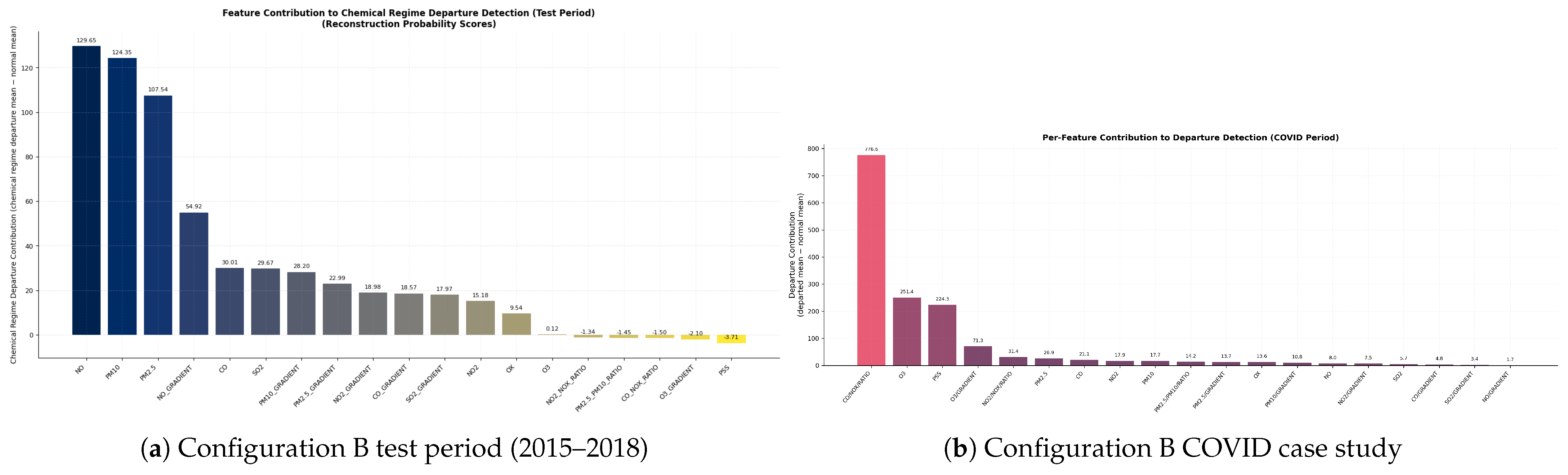
To test whether this COVID fingerprint is a property of the atmosphere or of the model, the COVID period was also analysed using Configuration B (trained 2011–2015), which produces an entirely different test-period profile dominated by raw concentrations (NO, PM10, PM2.5; Appendix A). Despite this, Configuration B’s COVID analysis converges on the same top three features: CO/NOx (776.6), O3 (251.4), and PSS (224.3). A model trained on 2011–2015 chemistry, which essentially represents a diesel-dominated traffic, higher NOx, and vigorous O3 titration, independently identifies the same atmospheric processes as disrupted during COVID as a model trained on 2015–2019 chemistry. This convergence confirms that the COVID atmospheric disruption has a characteristic multivariate fingerprint robust to the choice of training period: it is a property of the atmosphere, not an artefact of model specification. Configuration B shows a lower overall COVID departure rate (6.0%), consistent with its broader baseline encompassing a wider range of chemical variability. The full Configuration A vs. B test-period comparison is presented in Appendix A.
3.5. Meteorological and Temporal Attribution at Marylebone Road
The BRF classifier at MY1 achieves 78% overall accuracy with 79% recall for departed hours (Figure 11). Meteorological features account for 75.0% of total Gini importance, led by wind direction (0.352), air temperature (0.170), boundary layer height (0.133), and wind speed (0.094). The low importance of rush-hour (0.005) and weekend (0.010) indicators confirms that departures reflect structural emission composition changes rather than traffic-volume-driven events.
Figure 11.
BRF Gini feature importance at London Marylebone Road (MY1, 2022–2025). Meteorological features account for 75.0% of total importance, led by wind direction (0.352), air temperature (0.170), and boundary layer height (0.133). Rush-hour and weekend indicators contribute <1.5% combined.
The meteorological attribution (Figure 12) reveals physically coherent patterns. Departure rates show a U-shaped temperature response: elevated under cold conditions (35.8% at <0 °C; stable boundary layers concentrate the altered emission mix) and under very warm conditions (46.2% at 25–30 °C; intense photochemistry maximises the O3–NOx disruption). Low wind speeds promote departures (28.2% at 0–1 m/s; ), as do shallow boundary layers (31.5% at <100 m; , ). The near-flat diurnal profile (peak 15.1% at 01:00, trough 14.0% at 17:00) provides further evidence that departures are not rush-hour phenomena.
Figure 12.
Twelve−panel meteorological attribution analysis at London Marylebone Road (MY1, 2022–2025). Panels show departure rate as a function of: wind direction rose, wind speed, air temperature, boundary layer height (BLH), rates by wind speed bins, rates by temperature bins, rates by BLH bins, diurnal pattern, monthly pattern, annual evolution, BLH diurnal cycle, and departure rate by 16-sector wind direction. Meteorological features account for 75.0% of total BRF Gini importance.
The 16-sector wind rose analysis (Figure 13) reveals that NE winds produce 2.08× the baseline departure rate (, ) despite comprising only 12.2% of hours, while prevailing SW winds (23.3% of hours) produce the lowest rates (0.40×). Continental air masses from the NE–E sectors carry different VOC/NOx ratios and aged photochemical pollution that, upon mixing with local roadside emissions from the modernised fleet, produce multivariate pollution states that depart further from the baseline than the cleaner Atlantic air from SW flows. Thus, it is a significantly important finding that the departed wind sectors are in the exact opposite direction compared to the usual wind distribution across London.
Figure 13.
Wind rose analysis at MY1 for the 2022–2025 testing configuration. (a) Departure rate by sector. (b) Wind frequency. NE winds: 2.08× enrichment; prevailing SW winds: lowest rates.
3.6. Spatial Contrast: Roadside vs. Urban Background
The identical framework applied to London North Kensington (KC1, urban background; trained 2015–2019, tested 2022–2025) yields a fundamentally different departure profile. At KC1, the departure rate is 0.6% of sequences (2.2% of hours), with only 16 contiguous departure regions compared to 123 at Marylebone Road. The dominant contributors at KC1 (Figure 14a) are raw pollutant concentrations: CO (484.5), CO gradient (277.7), NO (145.6). The chemical ratios that dominate at Marylebone Road are negligible or negative at KC1: CO/NOx (−45.0), O3 (−9.3), and PSS ranks only 7th (56.0). This negative CO/NOx contribution indicates that the model actually reconstructs this ratio better during departed hours, meaning that the combustion fingerprint of fleet modernisation is not expressed at the background site. The per-pollutant classification confirms that KC1 departure hours show an average pattern/chemistry fraction of only 29.0% compared to 59.0% at MY1. These are overwhelmingly concentration-driven events reflecting how much pollution arrives, not what chemical form it takes.
Figure 14.
Per−feature departure contributions at North Kensington (KC1) (Training 2015–2019, Testing 2022–2025). (a) Test period: raw concentrations dominate; CO/NOx is negative (−45.0). (b) COVID: O3 dominates (271.4); CO/NOx (−0.9) and PSS (2.8) are negligible.
This spatial contrast has direct implications for evaluating the ULEZ and fleet modernisation policies. At the roadside, where fresh traffic emissions dominate, fleet modernisation directly alters the CO/NOx emission ratio and the local photostationary equilibrium. At the background site, these emission ratios have been diluted and chemically processed during transport, and the dominant departure signal shifts to absolute concentration changes. The combustion fingerprint of the policy intervention appears maximally expressed at the point of emission and does not appear to propagate to the single background monitoring station studied (KC1, North Kensington, approximately 3 km from the roadside). Whether this result generalises to other background sites or across the broader urban domain would require analysis of a denser monitoring network and is an important direction for future work.
3.6.1. Different Meteorological Controls at Different Sites
The BRF classifier at KC1 achieves 94% overall accuracy (Figure 15a), with a fundamentally different feature importance structure: air temperature dominates (0.294), followed by boundary layer height (0.202), while wind direction ranks only 5th (0.075). At MY1, wind direction leads (0.352). This reversal reflects different physical mechanisms: at the roadside, the direction of air arrival determines the source–receptor geometry; at the background site, atmospheric trapping controls accumulation. The boundary layer height effect is dramatically amplified at KC1 (mean 235 m departed vs. 657 m normal; , 3.5× the MY1 effect size of ). This is a crucial parameter in a background environment, since the boundary layer height is directly related to the total volume of the atmosphere. Similarly, temperature shows an 8.3 °C difference (2.8 °C departed vs. 11.1 °C normal, compared to only 1.6 °C at MY1). These results indicate that at a background site without a direct emission source, departures require extreme atmospheric trapping to concentrate transported pollution sufficiently for detection.
Figure 15.
Meteorological attribution at KC1 (Training 2015-2019, Testing 2022–2025). (a) Air temperature (0.294) and BLH (0.202) dominate, unlike MY1 where wind direction leads. (b) Departure rate by wind sector (left) and general wind frequency by wind sector (right).
3.6.2. COVID at the Background Site: Only the Photochemical Signal Propagates
During COVID at KC1, O3 becomes the single dominant contributor (271.4), while CO/NOx (−0.9) and PSS (2.8) are effectively zero (Figure 14b). This is the opposite of MY1, where CO/NOx (708.6) and PSS (419.1) dominate alongside O3 (197.2). The near-zero combustion fingerprint at KC1 during COVID confirms that the CO/NOx ratio, encoding instantaneous source composition, is homogenised during atmospheric transport. What KC1 detects instead is the downstream photochemical consequence: O3 accumulation from reduced NO titration across the urban area as a whole [27].
This result implies that the ULEZ and fleet modernisation interventions have their most direct atmospheric impact at the point of emission, where the altered combustion composition is maximally expressed. At background sites, these interventions manifest not through the combustion fingerprint but through the aggregate photochemical consequences of changed emissions across the urban canopy (Table 3) (Figure 16).
Table 3.
Spatial comparison of departure characteristics between London Marylebone Road (MY1, urban roadside) and North Kensington (KC1, urban background). The two sites show contrasting departure profiles, meteorological controls, and COVID signatures, reflecting the different atmospheric environments.
Figure 16.
Meteorological controls at KC1 (Training 2015-2019, Testing 2022-2025). (a) BLH: departed hours average 235 m vs. 657 m normal (). (b) Temperature: departed hours average 2.8 °C vs. 11.1 °C.
3.7. Validation
A comprehensive validation framework comprising five independent tests confirms the robustness of the detected departed pollution states and the reliability of the per-feature decomposition. Table 4 summarises the results. The synthetic perturbation test achieves 100% top-1 accuracy across all 19 features, confirming that when the analysis identifies CO/NOx or PSS as dominant, this reflects a genuine reconstruction error excess rather than architectural bias. The PSS relationship break test, shifting O3 by 1.5 without modifying NO or NO2, correctly identifies O3 (rank 1), Ox (rank 2), NO2/NOx (rank 3), and PSS (rank 4), demonstrating that the VAE has learned the chemical relationship structure. The temporal clustering test confirms that the observed 133-h maximum block and 123 blocks ≥24 h cannot arise from random labelling ().
Table 4.
Summary of validation tests for the ensemble departure detection framework.
4. Conclusions and Policy Implications
This study introduced a framework for detecting and diagnosing changes in the chemical character of urban atmospheric pollution applied to London’s evolving emission landscape from 2015 to 2025. The framework of this study identifies multivariate pollution states that have departed from an established baseline (2015–2019) and diagnoses which chemical relationships drive each departure across the COVID and post-COVID periods. The principal findings carry significant implications for both atmospheric science and air quality policy.
4.1. London’s Atmosphere Has Structurally Evolved
The central finding of this work is that the post-COVID atmosphere at London Marylebone Road is characterised by departed pollution states that are dominated by the CO/NOx combustion ratio and the photostationary state equilibrium, representing the complex chemical relationships rather than individual concentrations. This means that London’s fleet modernisation and the ULEZ have not merely reduced the quantity of pollution but have altered the fundamental chemical identity of the roadside atmosphere. The combustion fingerprint has shifted as the fleet transitions from diesel to petrol, hybrid, and electric vehicles, and the photochemical equilibrium between NO, NO2, and O3 has adjusted to changed NOx levels. This distinction between quantitative and qualitative atmospheric change is confirmed by the alternative configuration (Appendix A): the earlier period of gradual fleet renewal (2011–2018) produced concentration-driven departures with chemical ratios ranking last, while the post-ULEZ period produces ratio-driven departures with individual concentrations ranking lower. The nature of atmospheric change has itself changed in London Marylebone Road.
4.2. Different Interventions Produce Different Atmospheric Signatures
The COVID-19 lockdown serves as a natural experiment that distinguishes two modes of atmospheric disruption examined in this study. Fleet modernisation changes what is emitted, source composition of the atmosphere, producing a CO/NOx-dominated departure signal. The combustion fingerprint has shifted, but sufficient NOx remains for meaningful O3 titration. On the other hand, traffic collapse changes how the atmosphere processes what remains, representing shifts in the photochemical regime, producing a 3.2× increase in the O3 departure contribution as the removal of fresh NO suppresses the titration pathway. The framework distinguished these two types of disruptions without any prior guidance, but purely through the multivariate pollution fingerprint. Two independently trained models (2011–2015 and 2015–2019 baselines) converge on the same COVID signature despite producing opposite test-period profiles, confirming that this diagnostic capability is robust. Moreover, these findings align with previous studies that documented suppressed NO titration and enhanced ozone accumulation during COVID-19 lockdowns across European cities [26,28], as well as the global evidence for abrupt but pollutant-specific air quality responses to mobility restrictions [29].
4.3. Policy Impacts Propagate Differently at Different Spatial Scales
The spatial contrast between London Marylebone Road (urban roadside) and North Kensington (urban background) reveals that the ULEZ combustion fingerprint appears most strongly expressed at the point of emission and does not appear to propagate to the single background monitoring station studied (KC1, North Kensington). This conclusion is conditional on the two stations analysed; extending the analysis to a denser monitoring network would allow more general conclusions about spatial propagation across the urban domain. At the roadside region, CO/NOx dominates both the COVID and post-COVID period departures, where, at the background site, CO/NOx is effectively zero (−45.0 in the test period, −0.9 during COVID). Instead, the background site detects the concentration-driven departures under trapping conditions of the atmosphere (BLH effect size is 3.5× larger than at the roadside), and, during COVID, the downstream photochemical consequence of reduced NO titration (O3: 271.4 being the single dominant feature). These findings have direct implications for monitoring network design: roadside monitors are essential for evaluating whether fleet composition policies have altered the combustion fingerprint, while background monitors capture the aggregate photochemical and concentration consequences of changed emissions across the urban canopy. Neither site provides a complete picture of policy effectiveness on its own. It should also be noted that expanding the processed data library would increase the volume of information, resulting in a much higher resolution for interpreting policy impacts.
4.4. Implications for Air Quality Management
These findings suggest several concrete implications for urban air quality management:
- The ULEZ is working, but differently than concentration trends suggest. The conventional evidence for ULEZ effectiveness relies on declining NO2 concentrations. Our results show that the intervention has produced a bigger change: the combustion fingerprint of the vehicle fleet has been altered at the point of emission. This is a more fundamental indicator of policy success than concentration reduction alone, because it confirms that the source composition itself has changed, not merely that dispersion conditions have varied.
- Ozone management requires attention alongside NOx reduction. The progressive divergence of summer photochemistry from the baseline, evidenced by rising summer reconstruction errors and the 3.2× O3 enhancement during COVID, indicates that continued NOx reductions will increasingly shift the O3–NOx equilibrium toward higher ambient ozone at roadside sites. This is a well-known non-linearity in urban photochemistry [6], but our framework provides the first continuous, multivariate quantification of how far this equilibrium has already shifted from the pre-ULEZ baseline.
- Monitoring networks should be designed for multivariate assessment. The fundamental difference between the roadside and background departure profiles demonstrates that individual pollutant concentrations measured at any single site type cannot capture the full atmospheric response to emission control policies. A monitoring strategy that combines roadside sites (for combustion fingerprint assessment) with background sites (for aggregate photochemical and concentration assessment) and applies multivariate analysis would provide substantially more diagnostic information than current approaches.
- The framework provides early warning of atmospheric regime change. The year-over-year convergence of seasonal reconstruction errors indicates that the post-ULEZ atmosphere is approaching a new quasi-equilibrium. Monitoring the reconstruction probability score as a continuous metric, rather than only detecting threshold exceedances, could serve as an early indicator of when the atmosphere’s chemical character is evolving faster or slower than expected under ongoing policy implementation.
- The framework enables prospective identification of atmospheric stress conditions. The meteorological attribution reveals that departed pollution states are predictable from weather conditions: cold temperatures, shallow boundary layers, low wind speeds, and continental air mass origins collectively identify 75% of departures. Since weather forecasts are themselves highly accurate at 48–72 h lead times, the meteorological profile of departed states could be used to forecast when the post-ULEZ atmosphere is most likely to exhibit its altered chemical character. This is distinct from conventional air quality forecasting, which predicts concentration exceedances: our framework would instead forecast when the multivariate pollution relationships are most likely to depart from baseline, providing early warning of periods when the atmosphere’s chemical processing is most disrupted. For example, a forecast of sub-zero temperatures with northeasterly winds and boundary layer heights below 200 m would signal a high probability of a departed pollution state in which the altered CO/NOx combustion fingerprint is maximally expressed. This prospective capability could support targeted public health interventions and real-time policy evaluation.
4.5. Limitations and Future Work
The framework of this study relies on the assumption that the training-period atmosphere represents a stable baseline. The training period (2015–2019 for Configuration A) contains approximately nine months of early ULEZ Phase 1 effects (April–December 2019). This is expected to make the 97th-percentile detection threshold marginally conservative (inflated by early-ULEZ variance), tending toward underestimation of post-ULEZ departure rates. The cross-configuration validation with Configuration B confirms that the COVID-period feature rankings are robust to baseline choice; a dedicated sensitivity analysis cutting the training period at end-2018 remains a high-priority future experiment to directly quantify the effect of ULEZ Phase 1 on the detection threshold.
The absence of Volatile Organic Compound (VOC) measurements from standard AURN instrumentation creates an interpretive constraint on PSS and O3 departures: the model cannot distinguish whether shifts in the NO–NO2–O3 balance reflect changes in NOx alone or simultaneous perturbations in VOC levels. London Marylebone Road is operated in a VOC-limited photochemical regime. This ambiguity is most consequential for summer photochemical departures. The CO/NOx combustion ratio is not affected by this limitation as it encodes source composition rather than photochemical processing.
The spatial conclusions drawn in Section 3.6 are conditional on the two monitoring stations analysed. North Kensington is only a one urban background site approximately 3 km west of central London and may not be representative of other background environments closer to or further from major transport corridors. Future work will extend the chemical state framework to additional urban networks across multiple cities and countries; a ten-year atmospheric record from Ankara, Turkey, provides an immediate candidate for examining whether analogous policy-driven chemical regime shifts are detectable in contrasting regulatory and emission contexts. Such extensions would allow more general conclusions about how emission policy signals propagate across the urban domain and whether the diagnostic signatures identified here are transferable across contrasting urban environments.
The Isolation Forest operates on point-level hourly feature vectors, and therefore, cannot detect temporal pattern anomalies (e.g., unusual diurnal cycles where individual hourly values are within range). Such patterns are captured by the VAE methods; the ensemble design ensures that the temporal sensitivity of the VAE provides primary detection while classical methods provide corroborating evidence. A similar constraint applies to gradient feature Z-scores, which are computed without prior smoothing; the conservative 4 threshold and the ≥3 ensemble requirement mitigate noise-driven false positives, but a systematic smoothing sensitivity analysis is a direction for future methodological work. Additionally, a sensitivity test comparing departure rates and feature rankings between a 2018-cutoff training period and the current 2019-cutoff would quantify the impact of baseline non-stationarity on the detection results.
The per-feature decomposition identifies which chemical dimensions drive departures but does not directly attribute them to specific emission sources; source apportionment using receptor modelling techniques applied to the departed hours identified by this framework would provide complementary information. The framework is demonstrated at two London sites; its applicability to other cities with different emission landscapes, photochemical regimes, and monitoring configurations warrants further investigation, as demonstrated by recent spatiotemporal machine-learning approaches to urban ozone management at scale [30].
Supplementary Materials
The following supporting information can be downloaded at: https://www.mdpi.com/article/10.3390/atmos17060589/s1, Supplementary Materials.py.
Author Contributions
Conceptualisation, A.E.; methodology, A.E. and M.A.H.K.; software, A.E.; validation, A.E.; formal analysis, A.E.; investigation, A.E., D.T. and A.B.; data curation, A.E.; writing—original draft preparation, A.E.; writing—review and editing, A.E., D.T., A.B., D.E.S. and M.A.H.K.; visualisation, A.E.; supervision, D.T., A.B. and D.E.S. All authors have read and agreed to the published version of the manuscript.
Funding
This research received no external funding.
Institutional Review Board Statement
Not applicable.
Informed Consent Statement
Not applicable.
Data Availability Statement
Air quality monitoring data from the Automatic Urban and Rural Network (AURN) are publicly available from the UK Department for Environment, Food & Rural Affairs (DEFRA) at https://uk-air.defra.gov.uk/, accessed on 27 May 2026. ERA5 reanalysis data are available from the Copernicus Climate Change Service at https://cds.climate.copernicus.eu/, accessed on 27 May 2026. The Python code implementing the VAE ensemble framework is provided as Supplementary Material and will be deposited to a public repository (GitHub) upon acceptance.
Acknowledgments
During the preparation of this manuscript, the author used Claude (Anthropic), Opus 4 for the purposes of drafting and structuring the manuscript text. This work was supported by tools developed under NERC grant NE/V004069/1, along with data provided through NE/T001984/1. The author has reviewed and edited all output and takes full responsibility for the content of this publication. The author acknowledges DEFRA for maintaining the AURN monitoring network.
Conflicts of Interest
The authors declare no conflicts of interest.
Abbreviations
The following abbreviations are used in this manuscript:
| AURN | Automatic Urban and Rural Network |
| BLH | Boundary Layer Height |
| BRF | Balanced Random Forest |
| GRU | Gated Recurrent Unit |
| KC1 | London North Kensington (site code) |
| MAE | Mean Absolute Error |
| MY1 | London Marylebone Road (site code) |
| PSS | Photostationary State |
| ULEZ | Ultra Low Emission Zone |
| VAE | Variational Autoencoder |
Appendix A. Configuration A vs. B: Two Modes of Atmospheric Change
To assess whether the ratio-dominated departures observed in Configuration A (trained 2015–2019, tested 2022–2025) reflect a genuine qualitative shift in atmospheric pollution relationships or merely the passage of time, the identical framework was applied to an earlier period: Configuration B, trained from 2011 to 2015 and tested from 2015 to 2018.
The results (Figure A1a) reveal a fundamentally different departure profile. In Configuration B, the dominant features are raw pollutant concentrations: NO (129.7), PM10 (124.4), and PM2.5 (107.5), followed by the NO gradient (54.9). Chemical ratios, the features that dominate Configuration A, rank at the very bottom of the contribution list, with all showing negative or near-zero values: CO/NOx (−1.5), PSS (−3.7), O3 gradient (−2.1), NO2/NOx ratio (−1.3), and O3 itself contributes only 0.12. The ≥3 ensemble departure rate is 0.3% of sequences, nearly an order of magnitude lower than the 2.2% in Configuration A, corresponding to 1.6% of hours vs. 14.5%.
Figure A1.
Per−feature departure contributions for Configuration B (trained 2011–2015). (a) Test period (2015–2018): raw concentrations dominate; chemical ratios show negative contributions. (b) COVID: the same top three features as Configuration A (CO/NOx, O3, PSS), confirming robustness.
The per-pollutant classification further sharpens this contrast. In Configuration B, the average pattern/chemistry fraction is only 37.2%, compared to 59.0% in Configuration A. Concentration-driven departures dominate: CO shows 63.8% high-concentration departures, PM10 shows 62.1%, and PM2.5 shows 62.8%.
This comparison demonstrates that the nature of atmospheric change at London Marylebone Road has itself changed over time. Between 2011 and 2018, pollutant amounts shifted, but their chemical relationships were largely preserved, a quantitative change in the pollution landscape. Between 2015 and 2025, the chemical relationships themselves transformed, a qualitative change. The combustion fingerprint (CO/NOx) and photochemical equilibrium (PSS) shifted in ways that the model, having learned 2015–2019 atmospheric chemistry, cannot reconstruct. This distinction would be invisible to any approach based on individual pollutant concentration trends alone.
The COVID cross-validation from Configuration B is presented in the main text (Section 3.4). Table A1 summarises the comparison.
Table A1.
Comparison of atmospheric change characteristics across the two configurations.
References
- Mudway, I.S.; Kelly, F.J.; Sheridan, S.; Holgate, S.T. London’s Ultra Low Emission Zone: Health and air quality effects. Lancet Public Health 2023, 8, e62–e63. [Google Scholar]
- Carslaw, D.C.; Murrells, T.P.; Andersson, J.; Keenan, M. Have vehicle emissions of primary NO2 peaked? Faraday Discuss. 2016, 189, 439–454. [Google Scholar] [CrossRef] [PubMed]
- Higham, J.E.; Ramírez, C.A.; Green, M.A.; Morse, A.P. UK COVID-19 lockdown: 100 days of air pollution reduction? Air Qual. Atmos. Health 2021, 14, 325–332. [Google Scholar] [CrossRef]
- Grange, S.K.; Carslaw, D.C. Using meteorological normalisation to detect interventions in air quality time series. Sci. Total Environ. 2019, 653, 578–588. [Google Scholar] [CrossRef]
- Kroll, J.H.; Heald, C.L.; Cappa, C.D.; Farmer, D.K.; Fry, J.L.; Murphy, J.G.; Steiner, A.L. The complex chemical effects of COVID-19 shutdowns on air quality. Nat. Chem. 2020, 12, 777–779. [Google Scholar] [CrossRef]
- Sillman, S. The relation between ozone, NOx and hydrocarbons in urban and polluted rural environments. Atmos. Environ. 1999, 33, 1821–1845. [Google Scholar] [CrossRef]
- Leighton, P.A. Photochemistry of Air Pollution; Academic Press: New York, NY, USA, 1961. [Google Scholar]
- Shi, Z.; Song, C.; Liu, B.; Lu, G.; Xu, J.; Van Vu, T.; Elliott, R.J.R.; Li, W.; Bloss, W.J.; Harrison, R.M. Abrupt but smaller than expected changes in surface air quality attributable to COVID-19 lockdowns. Sci. Adv. 2021, 7, eabd6696. [Google Scholar] [CrossRef]
- Carslaw, D.C. Evidence of an increasing NO2/NOx emissions ratio from road traffic emissions. Atmos. Environ. 2005, 39, 4793–4802. [Google Scholar] [CrossRef]
- Kingma, D.P.; Welling, M. Auto-Encoding Variational Bayes. In Proceedings of the 2nd International Conference on Learning Representations (ICLR), Banff, AB, Canada, 14–16 April 2014. [Google Scholar]
- An, J.; Cho, S. Variational autoencoder based anomaly detection using reconstruction probability. SNU Data Min. Cent. Tech. Rep. 2015, 2, 1–18. [Google Scholar]
- Park, D.; Hoshi, Y.; Kemp, C.C. A multimodal anomaly detector for robot-assisted feeding using an LSTM-based variational autoencoder. IEEE Robot. Autom. Lett. 2018, 3, 1544–1551. [Google Scholar] [CrossRef]
- Su, Y.; Zhao, Y.; Niu, C.; Liu, R.; Sun, W.; Pei, D. Robust anomaly detection for multivariate time series through stochastic recurrent neural network. In Proceedings of the 25th ACM SIGKDD, Anchorage, AK, USA, 4–8 August 2019; pp. 2828–2837. [Google Scholar]
- Hersbach, H.; Bell, B.; Berrisford, P.; Hirahara, S.; Horányi, A.; Muñoz-Sabater, J.; Nicolas, J.; Peubey, C.; Radu, R.; Schepers, D.; et al. The ERA5 global reanalysis. Q. J. R. Meteorol. Soc. 2020, 146, 1999–2049. [Google Scholar] [CrossRef]
- Pedregosa, F.; Varoquaux, G.; Gramfort, A.; Michel, V.; Thirion, B.; Grisel, O.; Blondel, M.; Prettenhofer, P.; Weiss, R.; Dubourg, V.; et al. Scikit-learn: Machine Learning in Python. J. Mach. Learn. Res. 2011, 12, 2825–2830. [Google Scholar]
- Cahuantzi, R.; Chen, X.; Güttel, S. A comparison of LSTM and GRU networks for learning symbolic sequences. In Proceedings of the Science and Information Conference, London, UK, 13–14 July 2023; pp. 771–785. [Google Scholar]
- Kingma, D.P.; Ba, J. Adam: A Method for Stochastic Optimization. In Proceedings of the 3rd International Conference on Learning Representations (ICLR), San Diego, CA, USA, 7–9 May 2015. [Google Scholar]
- Akiba, T.; Sano, S.; Yanase, T.; Ohta, T.; Koyama, M. Optuna: A next-generation hyperparameter optimization framework. In Proceedings of the 25th ACM SIGKDD, Anchorage, AK, USA, 4–8 August 2019; pp. 2623–2631. [Google Scholar]
- Liu, F.T.; Ting, K.M.; Zhou, Z.-H. Isolation forest. In Proceedings of the 8th IEEE ICDM, Pisa, Italy, 15–19 December 2008; pp. 413–422. [Google Scholar]
- Chen, C.; Liaw, A.; Breiman, L. Using Random Forest to Learn Imbalanced Data; Technical Report; University of California: Berkeley, CA, USA, 2004; Volume 110, pp. 1–12. [Google Scholar]
- Goodfellow, I.; Bengio, Y.; Courville, A. Deep Learning; MIT Press: Cambridge, MA, USA, 2016; pp. 108–120. [Google Scholar]
- Jenkin, M.E.; Davies, T.J.; Stedman, J.R. The origin and day-of-week dependence of photochemical ozone episodes in the UK. Atmos. Environ. 2002, 36, 999–1012. [Google Scholar] [CrossRef]
- Rodríguez, S.; López-Darias, J. Extreme Saharan dust events expand northward over the Atlantic and Europe, prompting record-breaking PM10 and PM2.5 episodes. Atmos. Chem. Phys. 2024, 24, 12031–12053. [Google Scholar] [CrossRef]
- Pope, R.J.; Sherwen, T.; Pazmino, A.; Shanber, M.; Arnold, S.R.; Chipperfield, M.P.; Crilley, L.R.; Doherty, R.; Feng, W.; Konovalov, I.B.; et al. Measurement report: MAX-DOAS measurements characterise Central London ozone pollution episodes during 2022 heatwaves. Atmos. Chem. Phys. 2023, 23, 7121–7139. [Google Scholar]
- Carslaw, D.C.; Farren, N.J.; Vaughan, A.R.; Drysdale, W.S.; Young, S.; Lee, J.D. The diminishing importance of nitrogen dioxide emissions from road vehicle exhaust. Atmos. Environ. X 2019, 1, 100002. [Google Scholar] [CrossRef]
- Sicard, P.; De Marco, A.; Agathokleous, E.; Feng, Z.; Xu, X.; Paoletti, E.; Rodriguez, J.J.D.; Calatayud, V. Amplified ozone pollution in cities during the COVID-19 lockdown. Sci. Total Environ. 2020, 735, 139542. [Google Scholar] [CrossRef]
- Holland, R.; Seifert, K.; Saboya, E.; Khan, M.A.H.; Derwent, R.G.; Shallcross, D.E. Elucidating the effects of COVID-19 lockdowns in the UK on the O3-NOx-VOC relationship. Atmosphere 2024, 15, 607. [Google Scholar] [CrossRef]
- Grange, S.K.; Lee, J.D.; Drysdale, W.S.; Lewis, A.C.; Hueglin, C.; Emmenegger, L.; Carslaw, D.C. COVID-19 lockdowns highlight a risk of increasing ozone pollution in European urban areas. Atmos. Chem. Phys. 2021, 21, 4169–4185. [Google Scholar] [CrossRef]
- Venter, Z.S.; Aunan, K.; Chowdhury, S.; Lelieveld, J. COVID-19 lockdowns cause global air pollution declines. Proc. Natl. Acad. Sci. USA 2020, 117, 18984–18990. [Google Scholar] [CrossRef]
- Ma, J.; Wang, Y.; Chen, H.; Liu, X.; Zhao, Z. NetGBM: A spatiotemporal gradient boosting machine framework for urban ozone prediction and health risk assessment. J. Geophys. Res. Atmos. 2024, 129, e2024JD041593. [Google Scholar] [CrossRef]
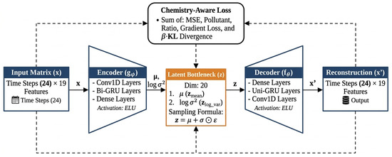
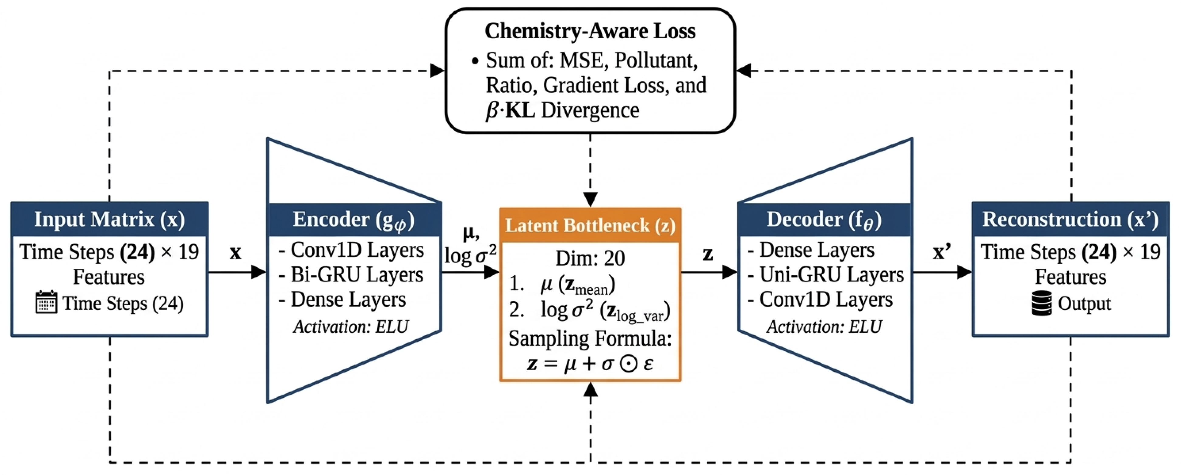
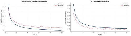
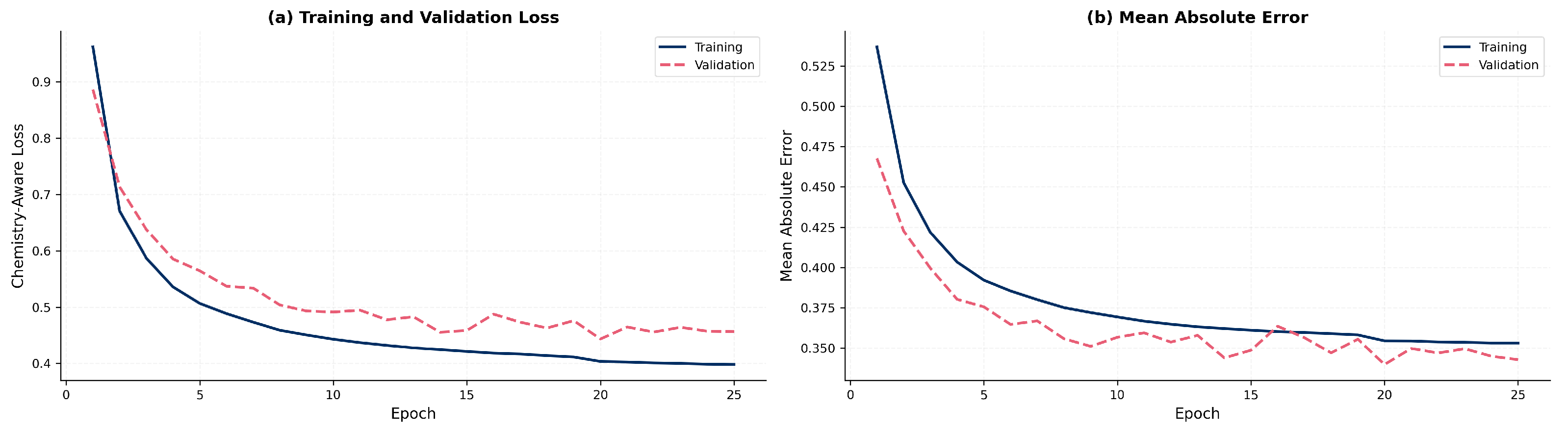
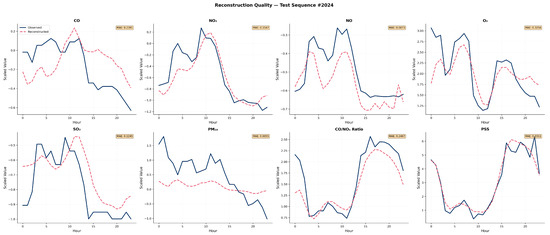
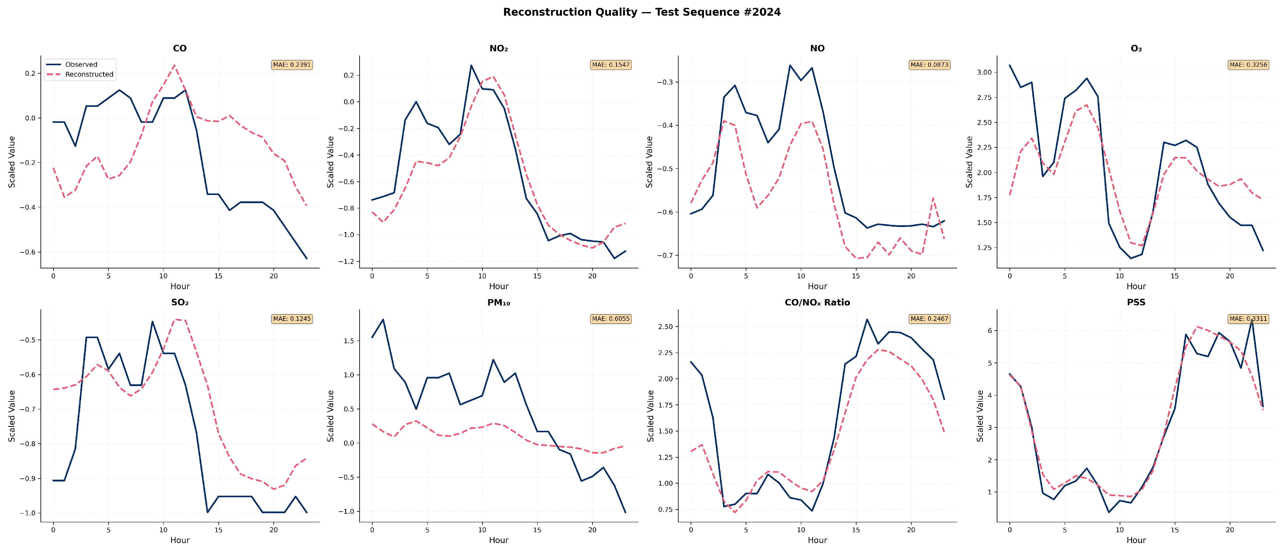
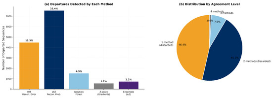
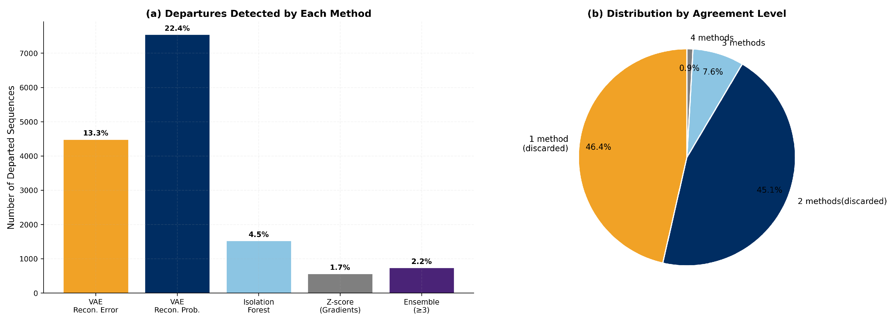
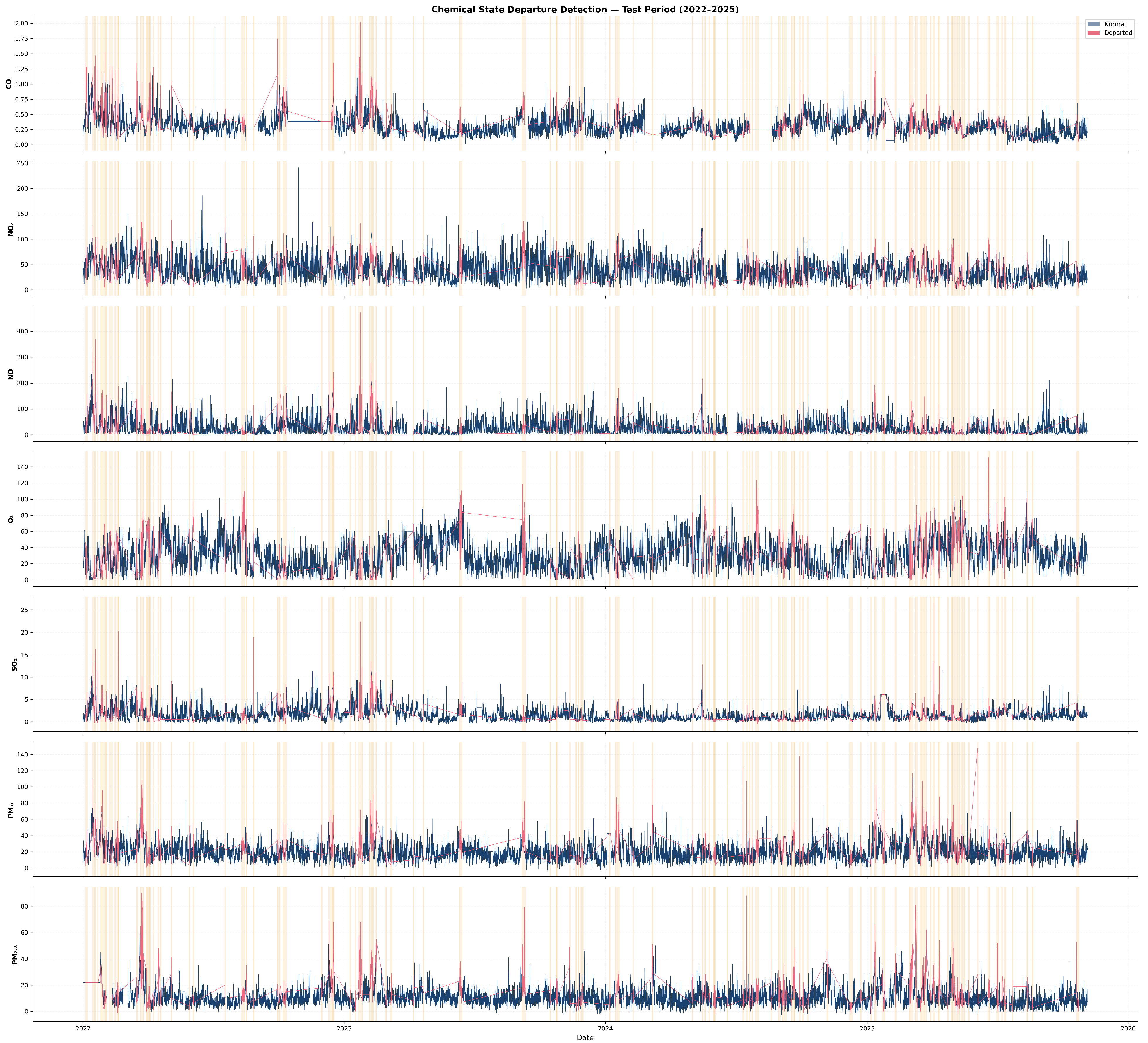
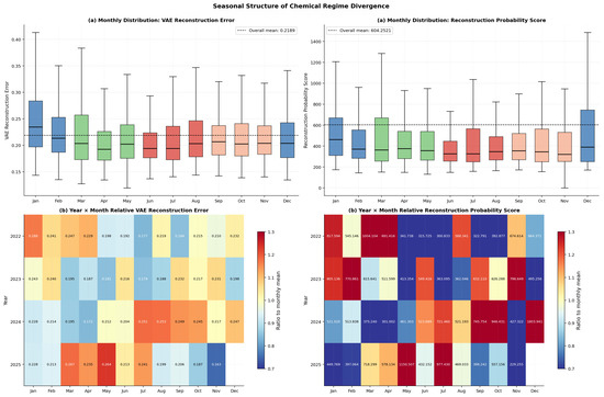
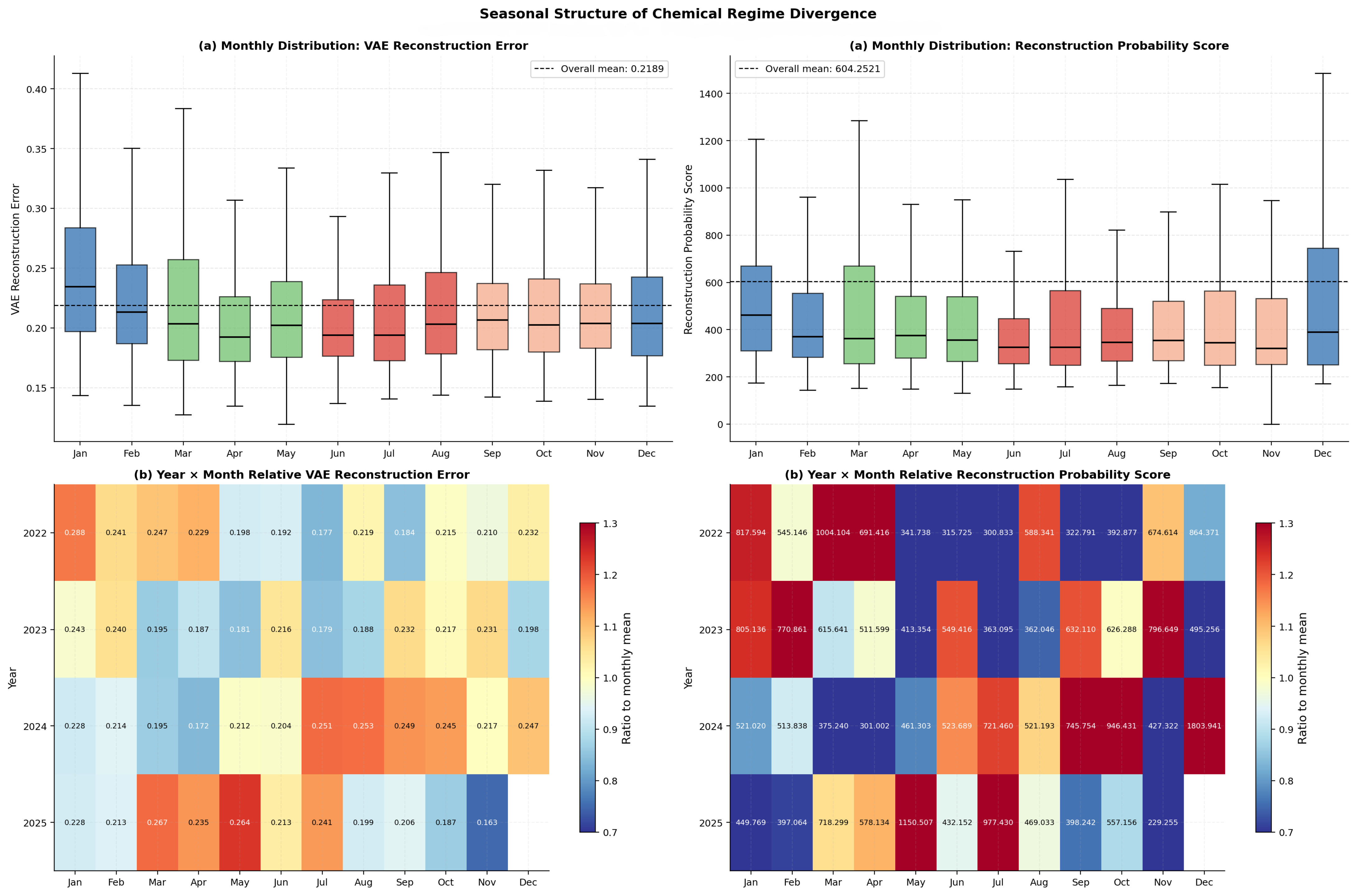
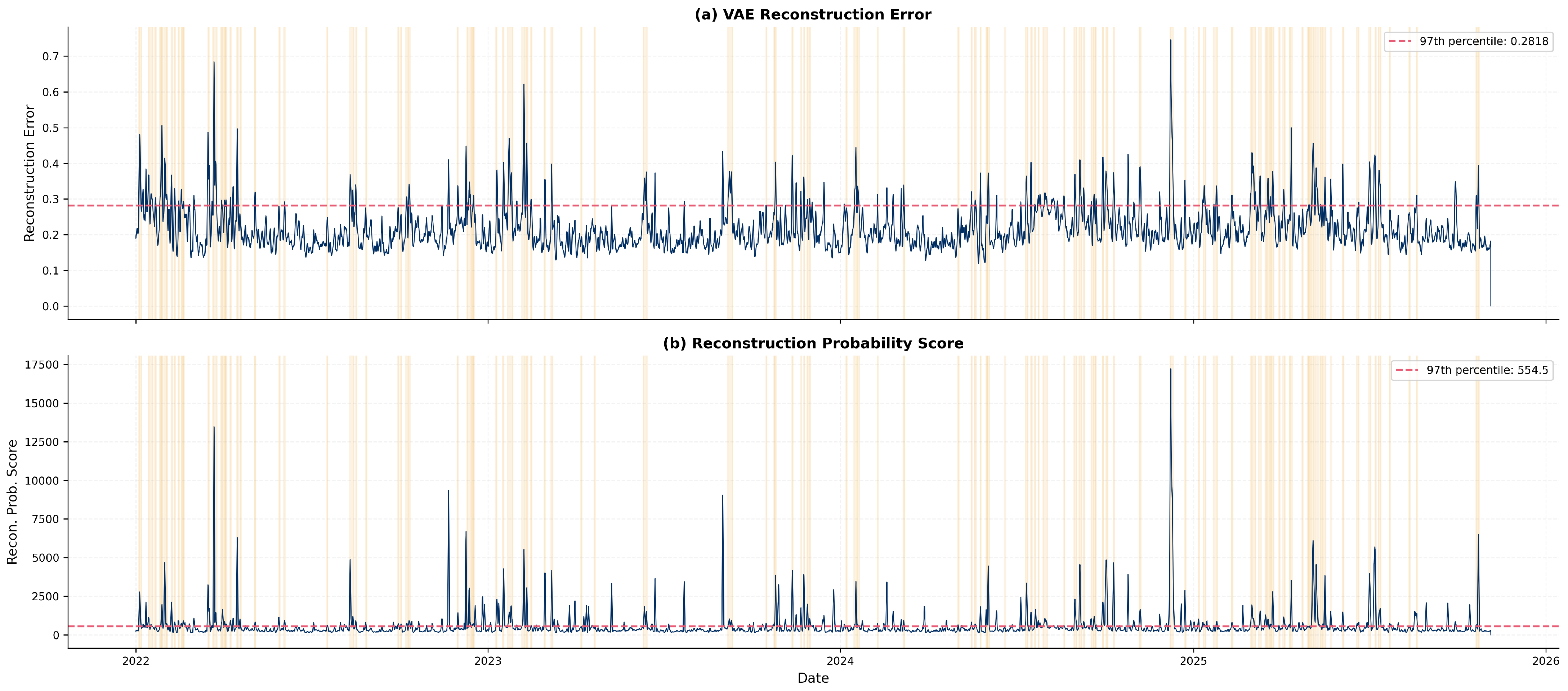
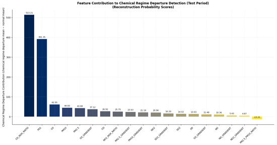
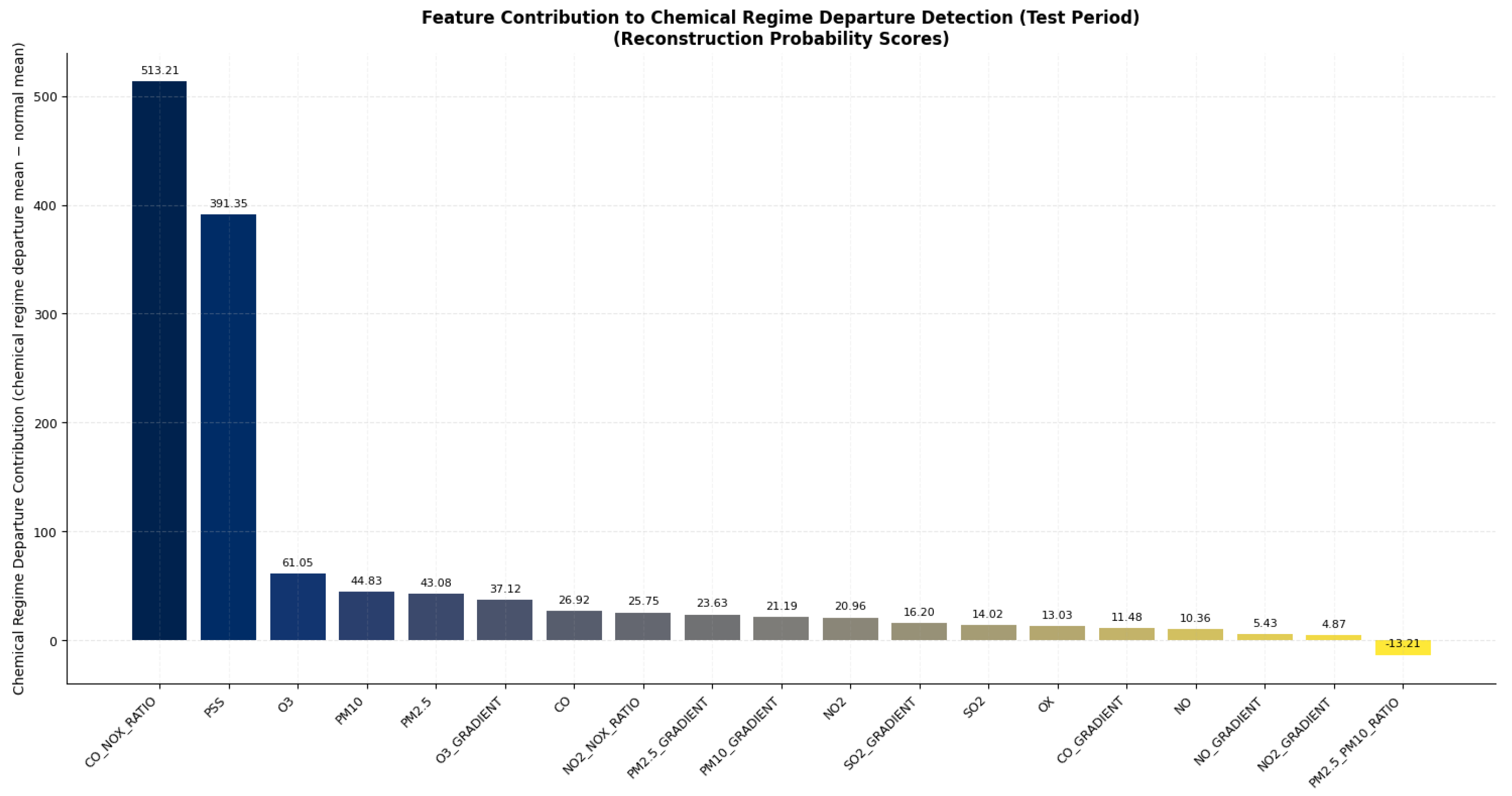
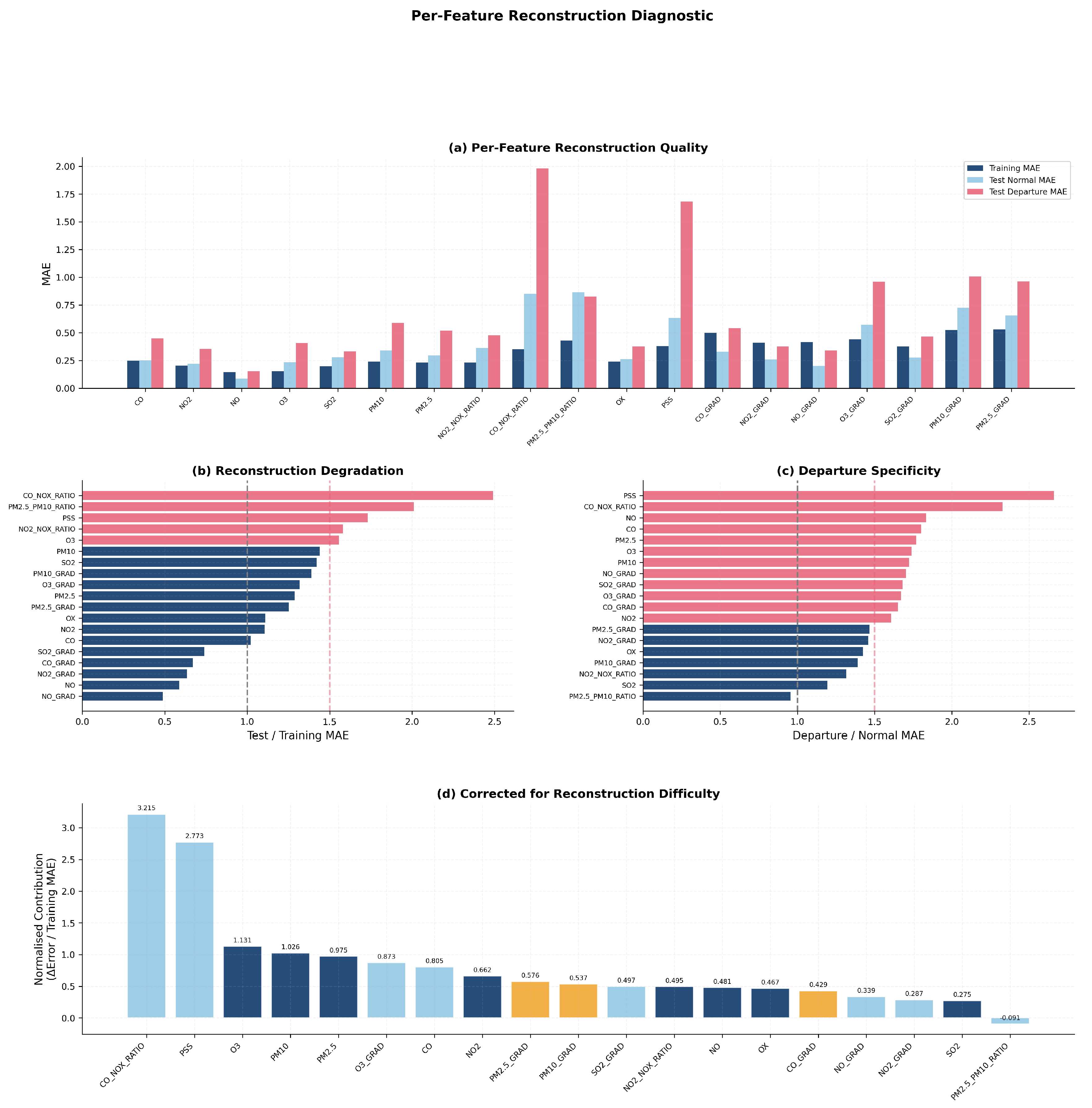
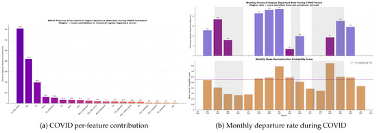
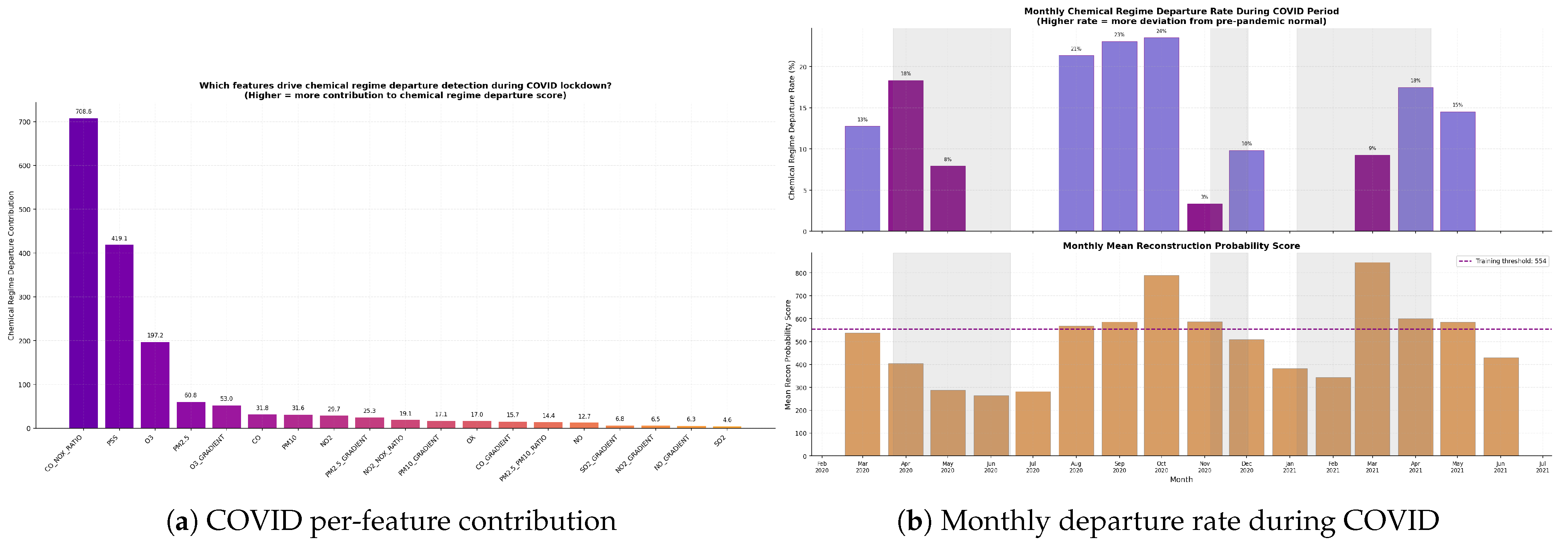
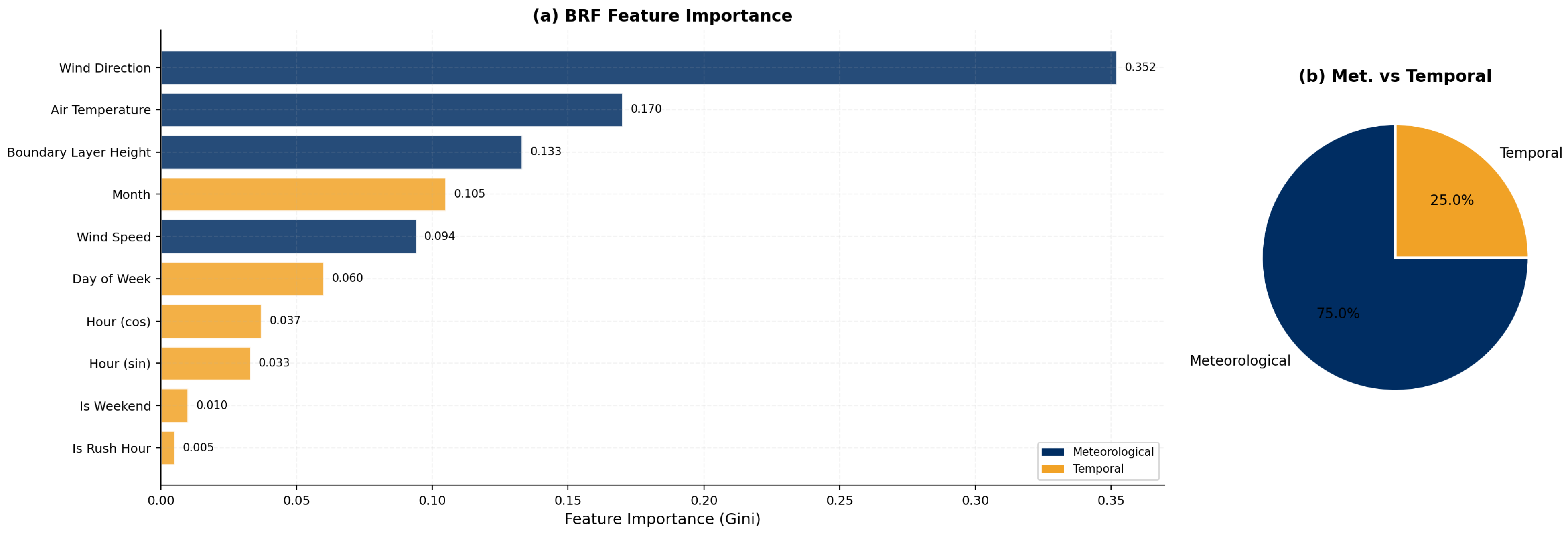
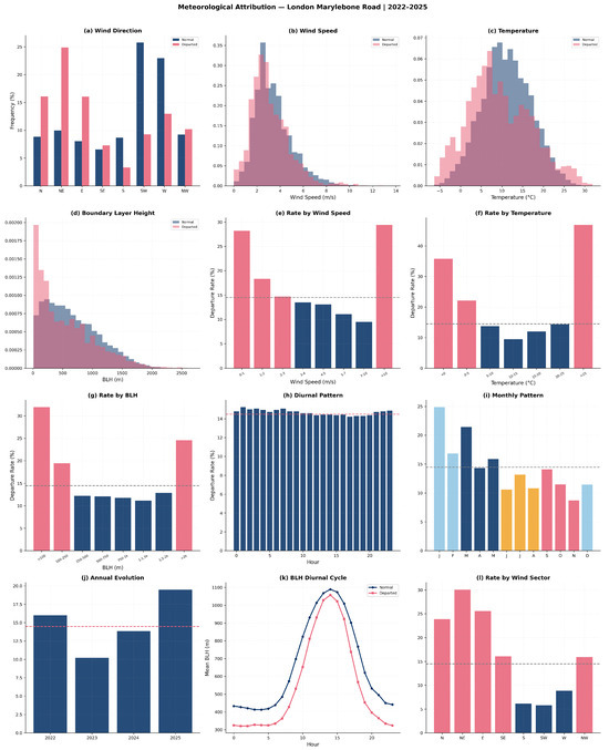
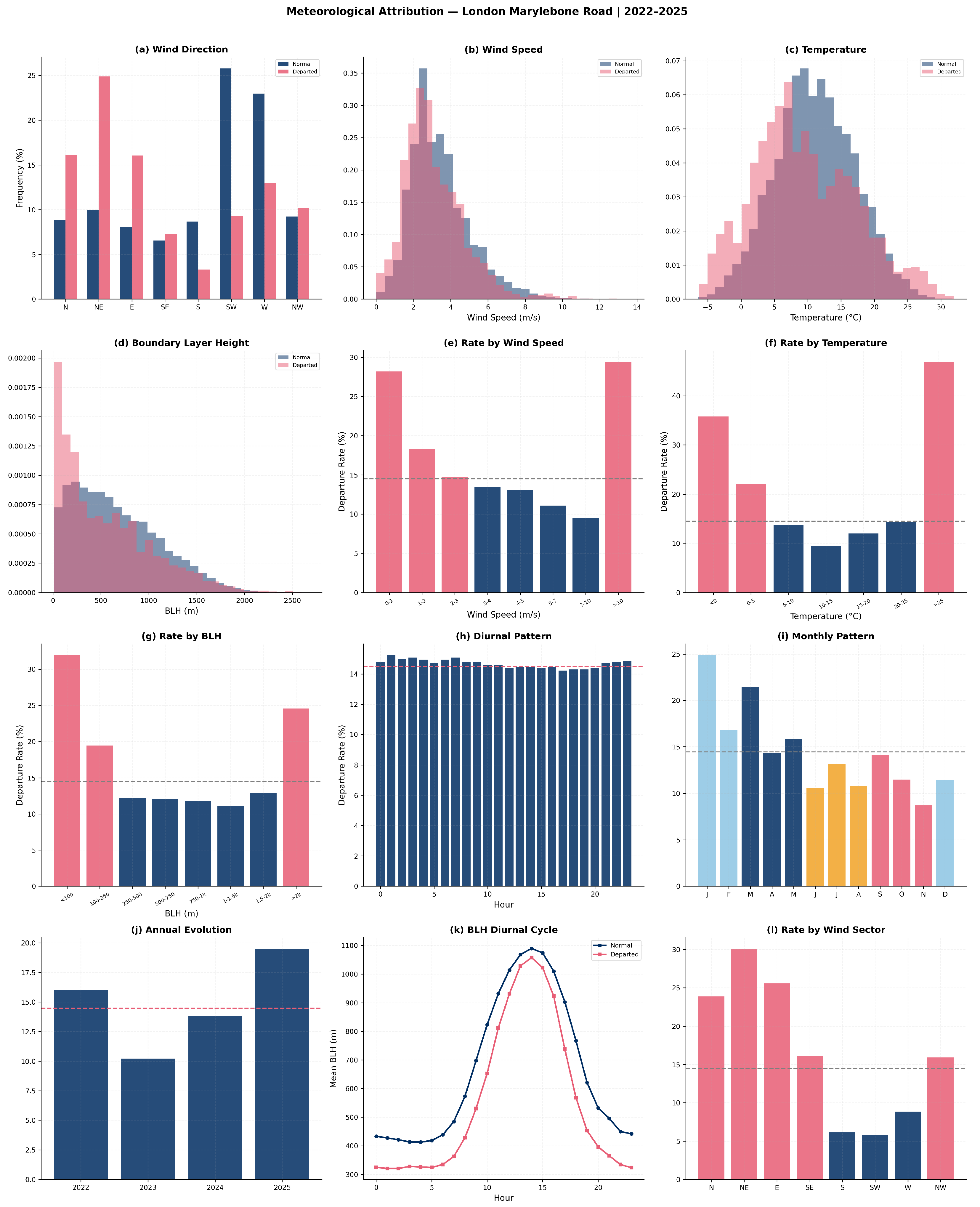
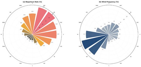
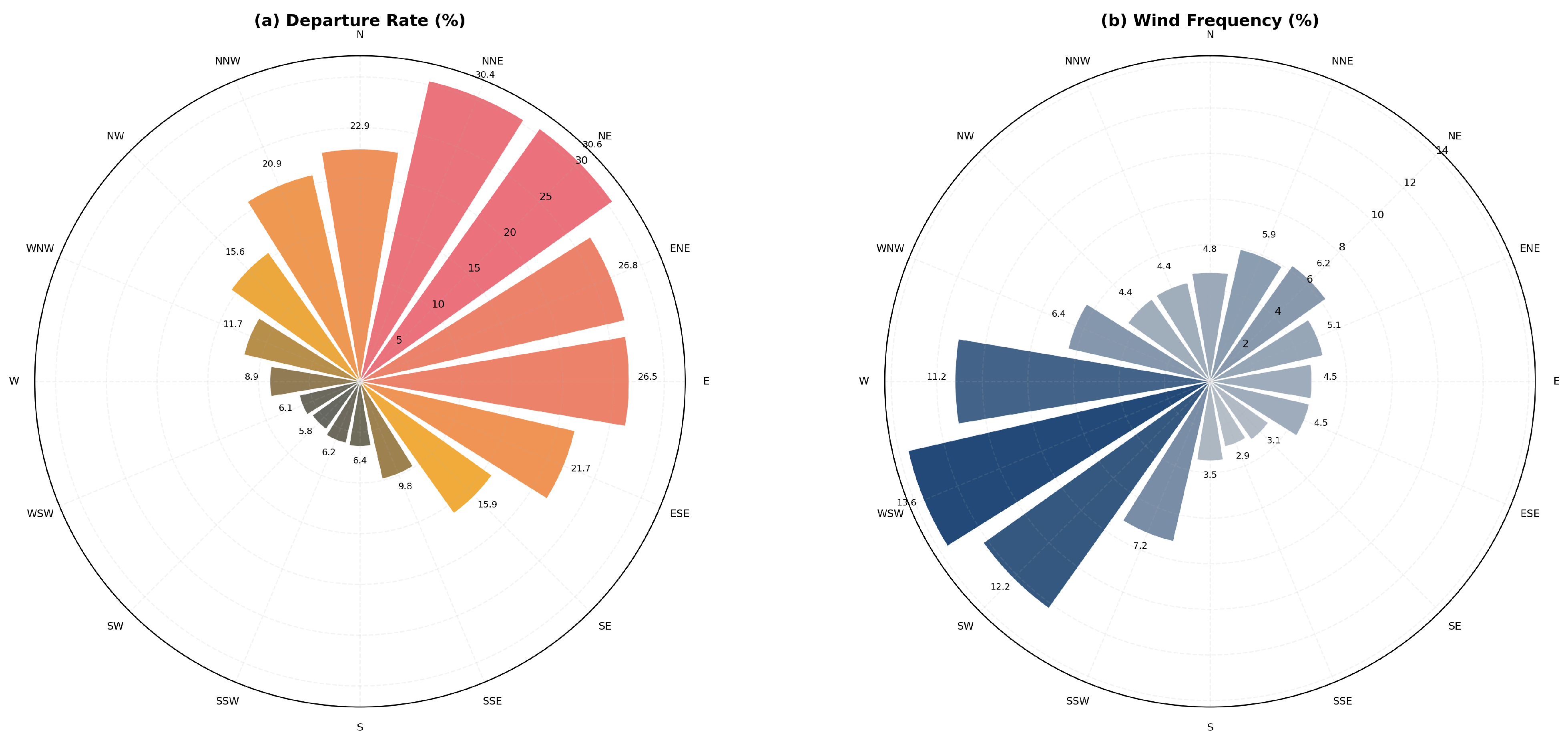
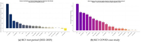
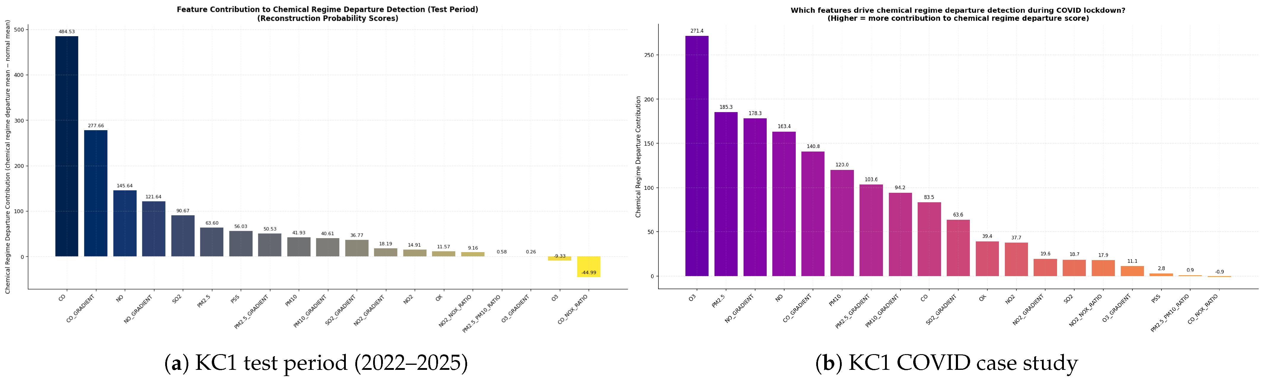
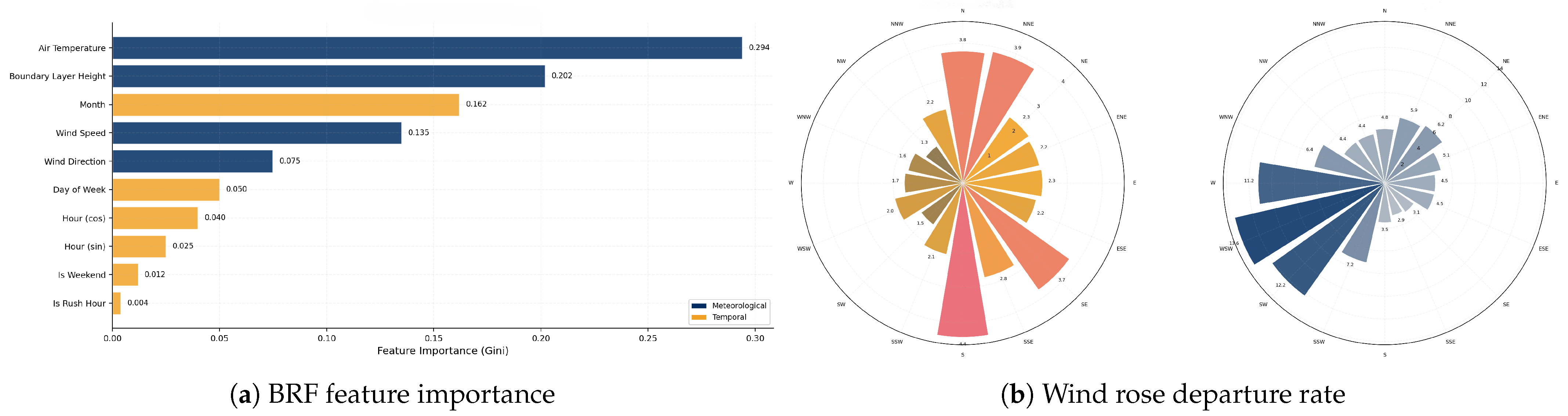
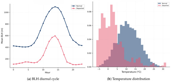
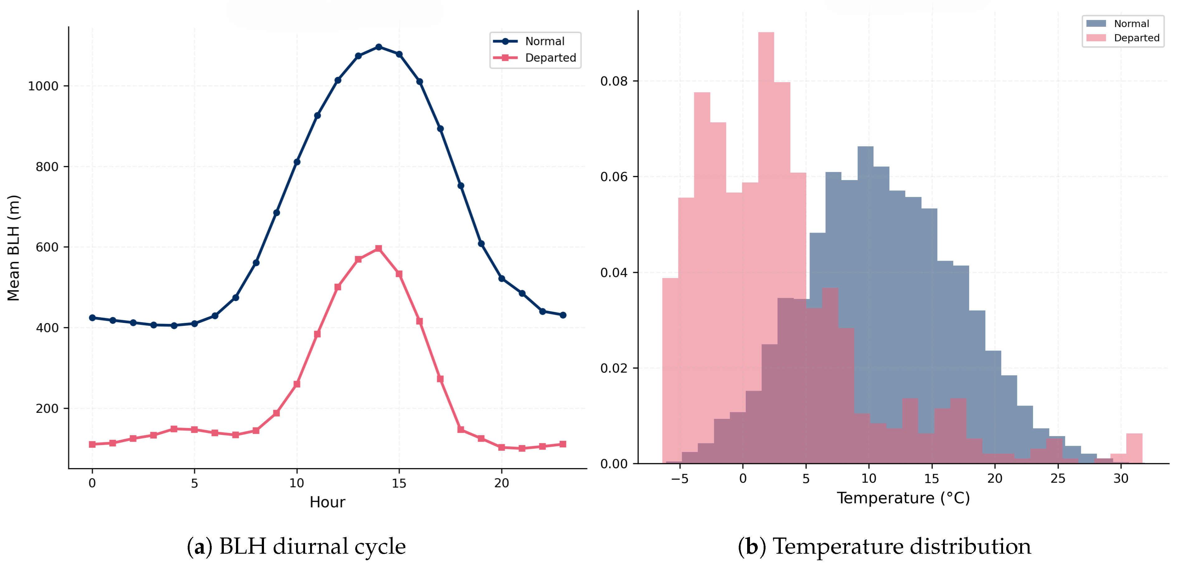

Disclaimer/Publisher’s Note: The statements, opinions and data contained in all publications are solely those of the individual author(s) and contributor(s) and not of MDPI and/or the editor(s). MDPI and/or the editor(s) disclaim responsibility for any injury to people or property resulting from any ideas, methods, instructions or products referred to in the content. |
© 2026 by the authors. Licensee MDPI, Basel, Switzerland. This article is an open access article distributed under the terms and conditions of the Creative Commons Attribution (CC BY) license.