


Abstract
Precipitation is among the most uncertain and poorly predicted weather products in earth system science. Local convective precipitation is particularly sensitive to strong land–atmosphere coupling. Two indices derived from atmospheric thermodynamic vertical profiles, convective triggering potential (CTP), a measure of the temperature lapse rate between approximately 1 and 3 km above the ground surface, and low-level humidity (HIlow), have become preferred measures of land–atmospheric coupling strength. To complement previous studies that primarily relied on limited station observations or regional analyses, this study provides a 20-year assessment of the CTP-HIlow framework for a wide area of the Continental United States (CONUS) using integrated satellite observations, reanalysis products, and surface datasets. The study further identifies important regional limitations in the framework’s predictive skill and demonstrates the influence of mid-level vertical wind shear on precipitation occurrence during both wet and dry soil advantage conditions. These findings provide new insight into why the framework performs inconsistently across different climate regions and suggest pathways for improving land–atmosphere coupling-based precipitation prediction. The objective is to determine the atmospheric and land-surface factors that control the regional performance of the CTP-HIlow framework and to identify how additional datasets that include more atmospheric variables can improve precipitation prediction skill.
1. Introduction
One of the most substantial unresolved modeling challenges in the field of earth system science concerns precipitation. The transfer of energy, moisture, and momentum between the terrestrial surface and the atmosphere, land–atmosphere coupling, when strong, is a significant factor in the formation of local convective precipitation [1]. It plays an essential function in the global climate system with significant effects on weather patterns, climate variability, and the water cycle. Depending on land-surface characteristics (e.g., vegetation cover, soil moisture, albedo, and roughness), meteorological conditions, diurnal and seasonal variations, among other influences, the intensity of land–atmosphere (L-A) coupling varies regionally, seasonally, and diurnally. It affects the duration and intensity of extreme weather events such as heavy rainfall [2,3,4], heat wave [5,6], and drought [7,8]. L-A coupling also plays a key role in climate modeling systems [9] including describing monsoon phenomena [10]. It is a significant challenge in furthering understanding of the weather and climate system, an issue that persists despite strong efforts over the decades [11,12].
Many metrics have been developed by the Global Energy and Water Exchanges (GEWEX) community [13]. Three of them which have been used for measuring the strength of L-A coupling are described here: soil moisture memory [14], the terrestrial coupling index (TCI; [14]), and the convective triggering potential (CTP)—low-level humidity index (HIlow) [1]. CTP is a measure of the temperature lapse rate between approximately 1–3 km above the ground surface; HIlow measures the humidity deficit in low-level air that becomes the daytime convective boundary layer. Since they depend on effective soil moisture content, these indices will vary from forested areas to grassland or agricultural regions. The CTP-HIlow index has become a preferred measure of land–atmospheric coupling strength. It has been developed over the NW USA but is often applied all over the entire CONUS. Over the last 20 years, researchers have documented a correlation between early-morning CTP-HIlow and afternoon precipitation on days manifesting classic convective boundary layer (CBL) structure. The CTP-HIlow framework defines the link between soil moisture and boundary layer interaction, in which early-morning measurements of CTP-HIlow have been used to identify locally triggered afternoon precipitation over soils with varying levels of moisture. Using a single-layer boundary layer model experiment and radiosonde observed datasets at Lincoln, Illinois [1], and over 89 stations across the United States [15], a framework has been developed. Using remote sensing datasets and an enhanced method for classifying days, ref. [16] applied the framework to seven years’ worth of climate data gathered from around the world. Ref. [17] examined CTP-HI and CDI using remote sensing (AIRS, AMSR-E). Ref. [18] established a classification scheme applicable to various datasets and regions, using soil moisture as a third dimension for drought in the southeastern United States. Different threshold values for CTP-HIlow have been proposed by [19] over the Tibetan Plateau (TP) based on boundary layer height and level of free convection, and it is given that a lower CTP can initiate convection over the TP due to its high altitude-induced air density and higher buoyancy. Combining the event frequency-based measurements of soil moisture–precipitation coupling with CTP-HIlow criteria in the central United States has revealed a consistently strong coupling between soil moisture and the partitioning of surface heat flux, and diurnal change in planetary boundary layer height [20].
Surface evaporative and sensible heat fluxes trigger summer convective rainfall in eastern US and northern Mexico, resulting in positive evaporation–precipitation feedback and effort expanded for all seasons by [21,22]. The success of incorporating the presence of low-level 3D winds into the CTP-HIlow framework suggests that convection occurs in a similar manner over different soils as noted using a previous framework for conditions of more convective intensity [23]. Numerous soil moisture datasets improve results [24], showing that observational research on soil moisture and precipitation interaction should always incorporate complementary information about the convective environment. Both positive and negative soil moisture feedback are important to describe convective activities observed in the Oklahoma Mesonet [25].
Land–atmosphere coupling strength is dependent on model configurations, including initialization time, model resolution, and most importantly, parameterization schemes [13,26,27]. Ref. [28] examined the land–atmosphere coupling strength in relation to the influences of afforestation and deforestation in the Weather Research Forecast (WRF) model during the European summer, concluding that extreme afforestation resulted in a weaker coupling using the CTP-HIlow framework. Modifying the vertical temperature and specific humidity profiles in WRF model outputs and the implementation of the CTP-HIlow framework revealed that the coupling strength and dominant signs of feedback are sensitive to temperature and humidity variations over Europe [28]. WRF simulations examining the influence of varying degrees of irrigated crop areas over the Southeastern United States indicate that the expansion of irrigation decreases near-surface temperature and increases near-surface humidity, resulting in a more stable boundary layer [29]. Using a soil moisture dataset of 40 km spatial resolution can help to initiate a cloud resolving model for mesoscale convective scale simulation [30], observing that the convection generally occurs around the peripheries of wet soil anomalies. Simulated surface precipitation is lower in moderately dry soils with an initial liquid water content slightly above the Permanent Wilting Point (PWP) than in the driest or wettest soils [31].
When the CTP-HIlow framework was first introduced, only the 2.5-degree NCEP-NCAR atmospheric reanalysis existed, and data storage and computing was still prohibitively expensive for high resolution climate modeling. Our aim here is to investigate scenarios in which the CTP-HIlow framework by itself is unable to adequately capture observed precipitation behavior. The objective is to determine what additional factors affect the framework’s performance and determine how these limitations might be overcome by adding complementary and higher-resolution input data. We begin by examining afternoon rainfall and CTP-HIlow threshold values at several FLUXNET locations in North America. Then, in the context of multiday weather sequences, locations where the CTP-HIlow criteria offer an insufficient or unclear representation of precipitation outcomes are identified and discussed. We aim to contribute to a more nuanced and balanced evaluation of the representativeness of the CTP-HIlow framework by highlighting situations in which other atmospheric and surface parameters are crucial.
2. Data and Methods
2.1. Data
2.1.1. AIRS Remote Sensing Data
The Atmospheric Infrared Sounder (AIRS) on board NASA’s Aqua satellite launched on 4 May 2002 “https://airs.jpl.nasa.gov/mission/overview/ (accessed on 12 April 2023)”. It provides data twice daily for each location, with equatorial crossings in local time at 1:30 a.m. (descending, or southward movement) and 1:30 p.m. (ascending, or northward movement), with a global repeat on the order of 2–3 days. Using a rotating mirror, AIRS performs sub-limb imaging in the across-track direction. The survey consists of 90 individual footprints and covers a ground distance of 1765 km for a 2.66 s scan. The distance between two readings is 18 km along the track. The AIRS V6 level 2 data is collected in “granules.” Each granule represents six minutes of measurement time, equivalent to 135 scans or 12,150 imprints. Along its length, a fragment measures 2430 km. The aperture of AIRS is 1.1, corresponding to a spatial resolution of 13.5 km at nadir. The period of orbit is 98.8 min. Its repeat cycle period is 233 orbits (16 days), amounting to repeatability on the ground of +/−20 km. The nominal orbital altitude is 705 km, with an inclination of 98.20° relative to the equatorial plane when viewed from the sun’s direction [32].
The AIRS V6 L3 gives 1° × 1° latitude/longitude gridded mean data all over the globe. The three different processing sets or variants of L3 products available are AIRS-only, AIRS + AMSU (Advanced Microwave Sounding Unit), and the AIRS + AMSU + HSB (Humidity Sounder for Brazil) [33]. Standard and support products are available for AIRS V6 data. We used the AIRS-only V6 L3 standard product. Quality control of all the parameters can be found in detail in [34]. Meteorological parameters used include geopotential height, water vapor mixing ratio at the surface and at pressure levels, surface pressure, and air temperature at surface and at other selected pressure levels. Temperature and water vapor mixing ratio data have been used for ten vertical levels, specifically the 1000, 925, 850, 700, 600, 500, 400, 300, 250, and 200 hPa levels. Fine cloud fractions at the 1018, 887, 771, 648, 548, and 447 hPa pressure layers have been used from AIRS-only V6 for the analysis. Comparing AIRS temperature and specific humidity with approximately 1500 National Climate Data Center (NCDC) data over the United States provides root mean square error (RMSE) values of 3.8 K and 32%, respectively [35].
2.1.2. ERA-5
The European Center for Medium-Range Weather Forecasts (ECMWF)’s next-generation reanalysis ERA5 is the improved version of ERA-Interim [36]. This new reanalysis data has many improvements such as spatial and temporal resolution, better representation of geophysical processes, and extensive observational inputs to the data assimilation system. ERA-5 data is at 0.25° latitude by 0.25° longitude spatial resolution and 1 h temporal resolution. This product has been used for comprehensive global simulations [37], and long-term simulations for climate studies [38].
For soil moisture analysis, volumetric soil water layer 1 (0–7 cm, the surface is at 0 cm) from ERA-5 has been considered. Other surface meteorological parameters at each hour such as total precipitation, surface temperature, surface pressure, and surface specific humidity, and vertical meteorological parameters such as horizontal and vertical winds, temperature, specific humidity, and geopotential height at the 1000, 925, 850, 700, 600, 500, 400, 300, 250, 200, and 200 hPa pressure levels have been used. These parameters have been used for both calculating CTP-HIlow and examining large-scale meteorological parameters.
2.1.3. NLDAS2
The North American Land Data Assimilation System (NLDAS-2) data is at 0.125° latitude by 0.125° longitude spatial resolution. In our analysis, NLDAS2 hourly precipitation data has been considered. All NLDAS-2 Noah soil moisture data is present at the following six levels, 0–10 cm, 0–40 cm, 0–100 cm, 0–200 cm, 10–40 cm, 40–200 cm, and soil moisture at the 0–10 cm layer has been considered in this analysis.
2.1.4. Automated Surface Observing Systems (ASOS) Stations
One of the primary weather observing systems in the United States is the ASOS, which provides standard meteorological measurements of humidity, temperature, wind speed and direction, pressure, sky condition, cloud fraction, precipitation, and visibility. These stations are supported and maintained by the Federal Aviation Administration, the National Weather Service, and the Department of Defense [39,40]. Most of the stations are located at airports so that data are used to make routine aviation weather reports (METARs). The ASOS ceilometer provides up to four cloud base heights and employs 0.9 µm lidar technology. We considered nine ASOS stations over North America selected on station proximity to AmeriFlux Core Sites “https://ameriflux.lbl.gov/sites/ameriflux-core-sites/ (accessed on 31 August 2023)”. Lower atmospheric meteorological parameters including the 2 m air temperature, 2 m dew point temperature, 2 m relative humidity, 10 m wind speed, cloud fraction, and surface pressure from ASOS stations were used “https://mesonet.agron.iastate.edu/request/download.phtml?network=AR__ASOS (accessed on 31 August 2023)”.
2.1.5. Site Selection
The final analysis was narrowed from the nine initial ASOS stations to four specific sites: ARM-SGP (Oklahoma), ARM-AMF3 (Alabama), Harvard Forest (Massachusetts), and Goodwater Creek (Missouri). Station selection required complete, continuous observational records spanning the entire 2002–2022 period. Additionally, these four locations were selected to capture the dominant land-surface types across CONUS, encompassing agricultural plains (SGP), mixed forest (AMF3 and Harvard Forest), and rain-fed cropland (Goodwater Creek). By spanning distinct climatological regimes including the semi-arid Southern Great Plains, the humid Southeast, the temperate Northeast, and the continental Midwest, this refined subset ensures a highly representative geographical sample across the United States.
Following a CONUS-wide climatological analysis of CTP-HIlow and large-scale meteorological parameters, we conducted an evaluation of local meteorological conditions at four selected ASOS stations (Table 1).
Table 1.
Period of wet soil and dry soil miss days over four METAR sites closest to ARM stations. No dry soil miss events were identified at HF during the study period, consistent with the climatologically humid conditions of the northeastern United States, where persistent forest cover, high mean summer precipitation, and frequent Atlantic moisture advection collectively suppress the occurrence of dry soil miss conditions as defined by the CTP-HIlow framework.
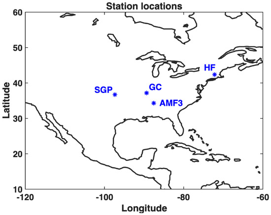
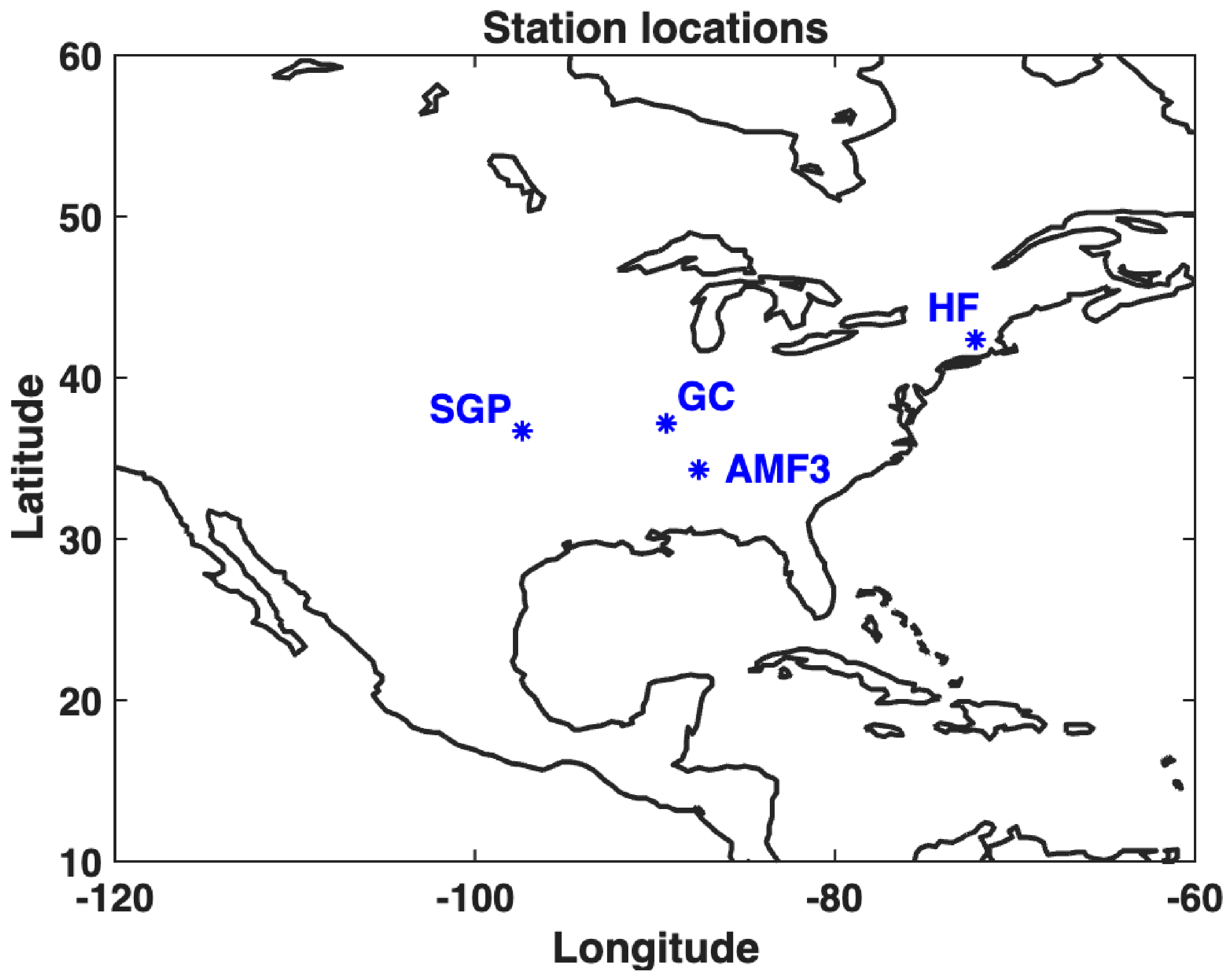
These stations (see map, Figure 1) include:
Figure 1.
Geographic locations of four stations used.
Orange Municipal Airport (ID: KORE), situated near Harvard Forest (HF) in Massachusetts, USA representing forested ecosystems in the northeastern United States. More than 90% of the Harvard Forest is closed-canopy forest. Almost all the forests in the region are second-growth, following millennia of stewardship by Indigenous people and then extensive agricultural clearing and logging that peaked in the mid-1800s (Harvard Forest: “https://harvardforest.fas.harvard.edu/research (accessed on 28 January 2024)”.
Blackwell-Tonkawa Airport (ID: KBKN), located adjacent to the Southern Great Plains (SGP) site in Oklahoma, USA characteristic of the southern U.S. plains region. Land use is primarily agricultural, including native prairie pasture, cropland, and pastureland “SGP: https://ltar.ars.usda.gov/sites/sp/ (accessed on 28 January 2024)”.
Haleyville Northwest Alabama Regional Airport (ID: K1M4), proximal to the third ARM Mobile Facility (AMF3) in Alabama, USA representing the southeastern U.S. forested terrain (Bankhead National Forest; “https://www.bnl.gov/newsroom/news.php?a=121671 (accessed on 28 January 2024)”; and Cape Girardeau Regional Airport (ID: KCGI), near Goodwater Creek (GC) in Missouri, USA a primarily agricultural site typical of the Midwestern United States. Land cover at GC is approximately 87% managed agricultural lands, 6% forests, and 7% urban [41].
2.2. Methods
To calculate CTP-HIlow, we used temperature and water vapor mixing ratio data from NASA’s Atmospheric Infrared Sounder (AIRS), and fifth generation ECMWF atmospheric reanalysis (ERA5). For soil moisture, and precipitation calculation ERA5 and NLDAS-2 data were used. METeorological Aerodrome Report (METAR) data have been used for in situ comparison.
2.2.1. Convective Triggering Potential (CTP)
The CTP (J kg−1) is a measure of atmospheric instability. It represents the deviation of the modeled temperature profile (Tenv) from the moist adiabatic lapse rate between 100 and 300 hPa (around 2000 m layer interval) above ground [16].
where “Zpsfc − 300” and “Zpsfc − 100” represent the height at surface pressure “Psfc − 300”, and “Psfc − 100”. “Tparcel” represents the temperature of an air parcel, which is lifted along the moist adiabatic lapse rate originating from 100 hPa above the surface and “g” is the gravitational acceleration. The lower free troposphere close to the top of the convective boundary layer, an area crucial for cloud initiation, is sampled by the 100 mb layer used in the CTP definition. It is intended to capture the thermal stratification that controls boundary layer growth toward the lifting condensation level and the possibility of shallow cloud formation, despite being somewhat shallower than a normal afternoon boundary layer. Thus, the lapse rate during this time span links boundary layer evolution to precipitation potential and offers a physically meaningful indicator of whether surface-driven turbulence can facilitate cloud formation and convective initiation.
Physically, a high positive CTP (0–200 J kg−1) indicates conditional stability in which the convective boundary layer can grow sufficiently to overcome the capping inversion and trigger precipitation. In contrast, a negative CTP indicates a strong inversion that suppresses convection initiation.
2.2.2. Low-Level Humidity Index (HIlow)
The HIlow (°C) corresponds to the sum of dew point depressions at 50 and 150 hPa above ground [15].
where “Tsfc − 50” and “Td,sfc − 50”are temperature and dew point temperature at 50 hPa above ground respectively. Similarly “Tsfc − 150” and “Td,sfc − 150” are temperature and dew point temperature at 150 hPa above ground respectively. The 50 hPa and 150 hPa above-ground levels used in HIlow correspond to the distance that boundary layer air must ascend and saturate before cloud formation can occur. A low HIlow (<10 °C) suggests that the lower troposphere is close to saturation and a high HIlow (>15 °C) suggests a moisture deficit atmosphere.
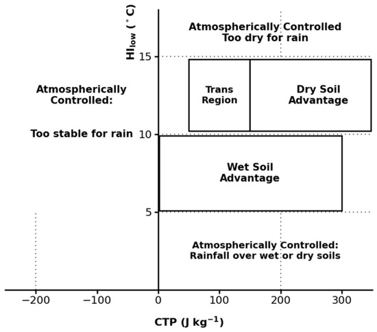
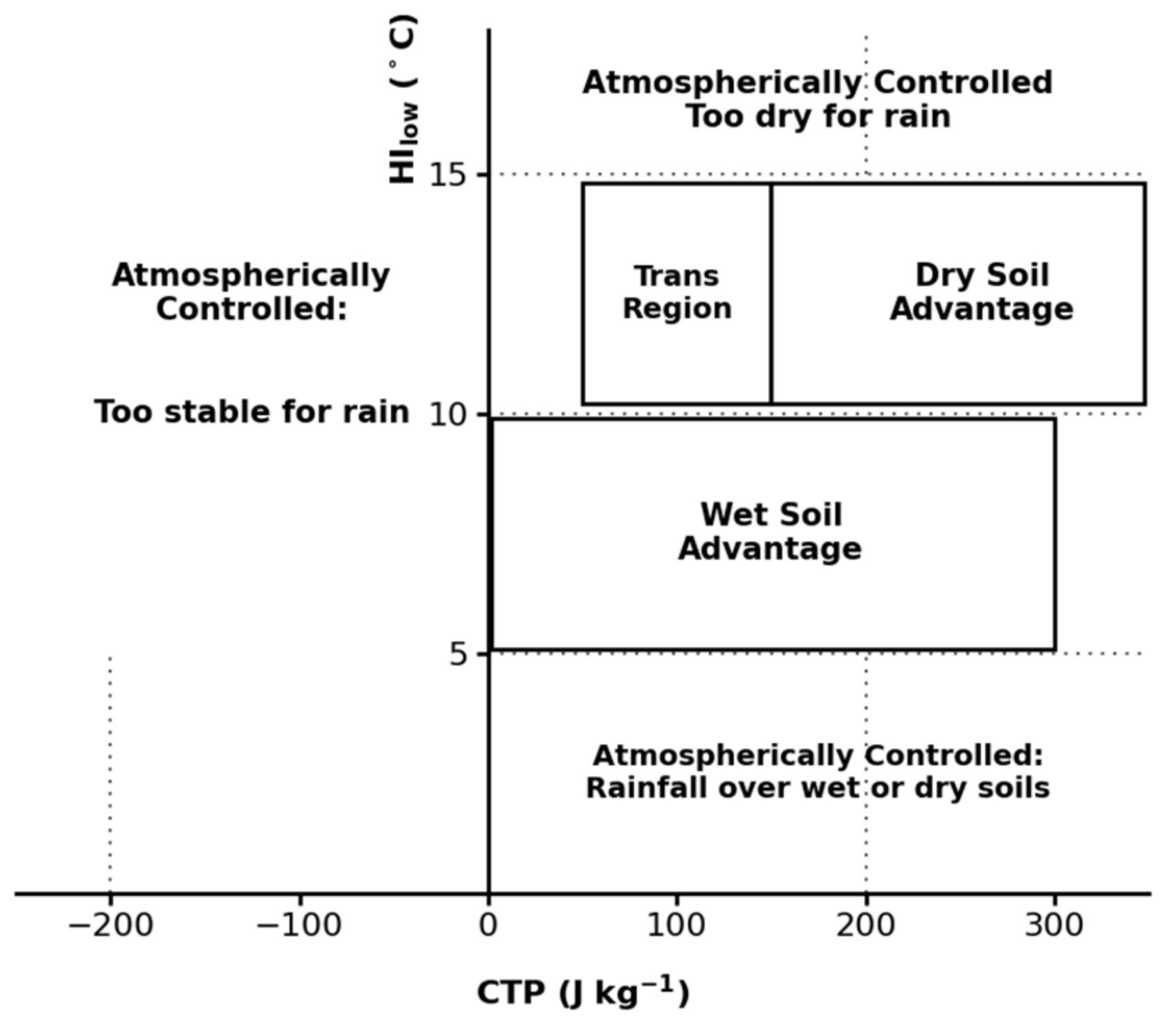
Together, CTP and HIlow define a two-dimensional diagram (Figure 2) that classifies each early-morning sounding. This framework originally developed by Findell and Eltahir (2003) was extended by [15]. Following the Ferguson and Wood (2011) [16] classification, four different regimes were used. (1) Atmospherically controlled—too dry for rain, where HIlow is greater than 15 °C; (2) atmospherically controlled—too stable for rain, where CTP is less than 0 J kg−1; (3) atmospherically controlled—rainfall over wet and dry soils, when CTP > 200 J kg−1 and HIlow < 15 °C; and (4) land-surface-controlled regime—when 0 < CTP < 200 J kg−1 and HIlow < 15 °C, the atmosphere is conditionally stable and the lower atmosphere is moist enough to support cloud formation, thereby governed by soil moisture content. This 4th regime, a zone of strong L-A coupling, is further divided into wet soil advantage and dry soil advantage.
Figure 2.
The CTP–HIlow framework for categorizing early-morning atmospheric profiles into four convective regimes: atmospherically controlled (too dry for rain; too stable for rain; rainfall over wet or dry soils regardless of surface state), wet soil advantage, dry soil advantage, and transition region (as reproduced in [16]).
2.2.3. Classification of Wet and Dry Soil Advantage Days
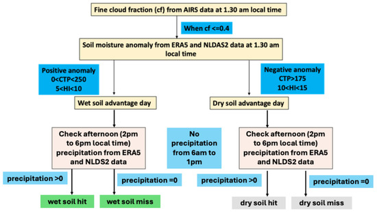
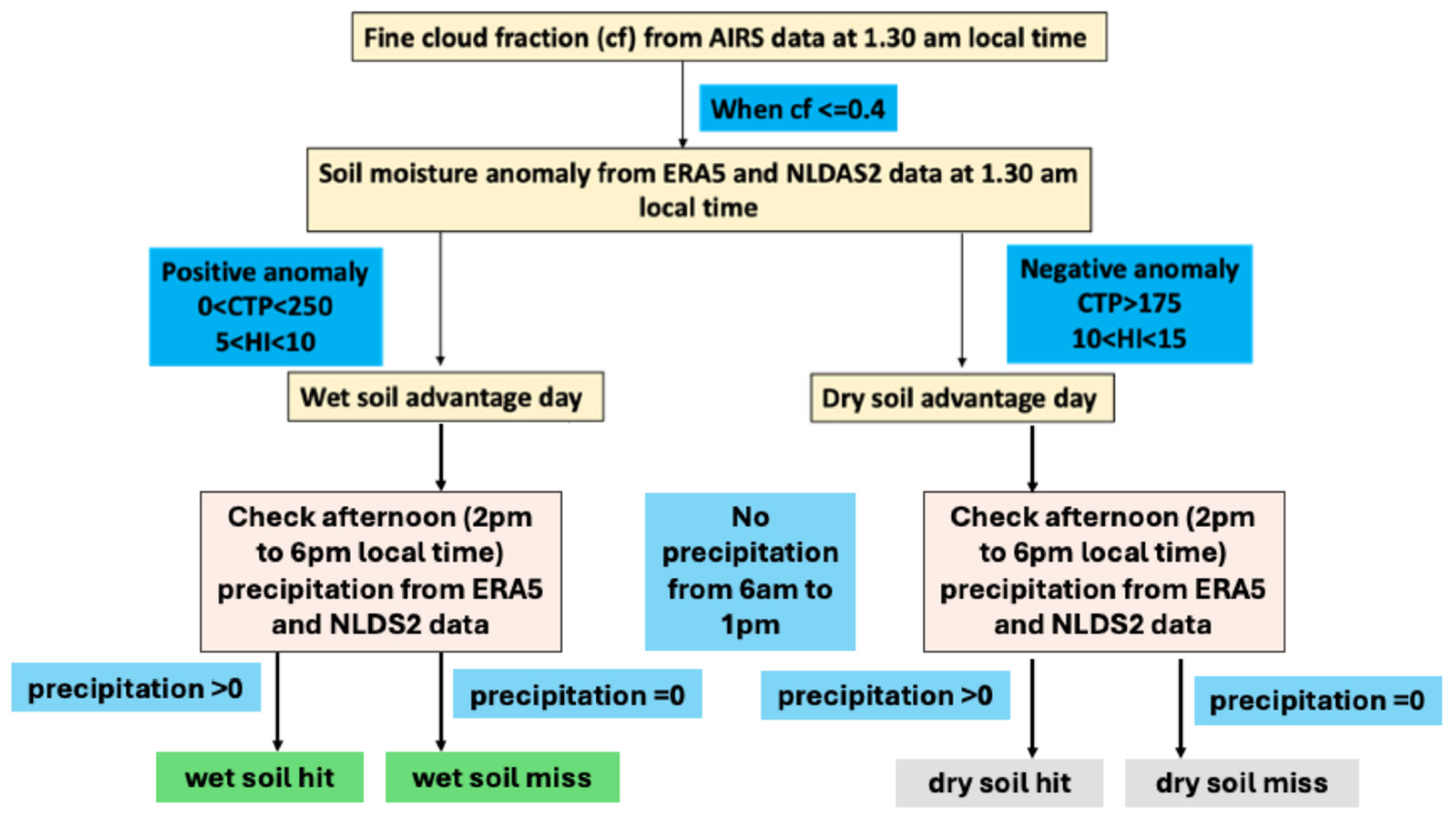
The detailed methodology (Figure 3) shows how using the Findell 2003a [15] threshold values for CTP and HIlow parameters, and wet and dry soil advantage days were classified. A fine cloud fraction ≤0.4 [15] was considered to be when there was no cloud present in each vertical layer in the early morning (1:30 a.m. local time) each day from AIRS data. The soil moisture and precipitation variables from ERA5 and NLDAS-2 datasets were regridded to the 1° AIRS spatial resolution using triangulation-based linear interpolation, implemented via MATLAB (2021a)’s “griddata” function. This method constructs a Delaunay triangulation from the source grid coordinates and interpolates soil moisture values onto the target 1° grid using linear weighting within each triangular element. Then it is adjusted to local time (LT). To check wet and dry soil advantage cases, the soil moisture anomaly at 1:30 a.m. LT was used. It was computed as the difference in each day at 1:30 a.m. local time and the average of the 30-day window centered on that calendar day of 30 years (1993–2022; Ford et al. 2023 [18]).
Figure 3.
Detailed flowchart of the methodology.
When there is no cloud fraction at 1:30 a.m. local time in AIRS data, positive soil moisture anomaly at 1:30 a.m. local time from corresponding ERA5 and NLDAS2 data, CTP varies from 0 to 250 J/kg, and HIlow varies from 5° to 10 °C, then the day has been classified as a wet soil advantage day. Similarly, when there is no cloud fraction at 1:30 a.m. local time in AIRS data, negative soil moisture anomaly at 1:30 a.m. local time from corresponding ERA5 and NLDAS2 data, CTP is more than 175 J/kg, and HIlow varies from 10° to 15 °C, then the day has been classified as dry soil advantage day.
After classifying wet and dry soil advantage days, afternoon precipitation for those days was examined. Initially, days with rainfall occurring in the morning half (i.e., between 6 a.m. and 1 p.m. local time) were excluded from the analysis, as such rainfall may have resulted from large-scale disturbances. Then, other days with wet/dry soil advantage have been checked for afternoon precipitation (i.e., 2 p.m. to 6 p.m.). If wet (dry) soil advantage days have no rainfall for both morning and afternoon times, then they are classified to be a wet (dry) soil miss. Similarly, if wet (dry) soil advantage days have rainfall in the afternoon, then they are taken as wet (dry) soil hit.
3. Results and Discussions
3.1. CONUS-Wide Performance of the CTP-HIlow Framework
3.1.1. Composite Mean Occurrence of Wet and Dry Soil Advantage Days over CONUS
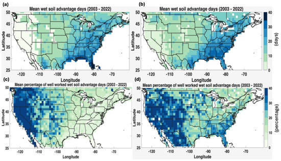
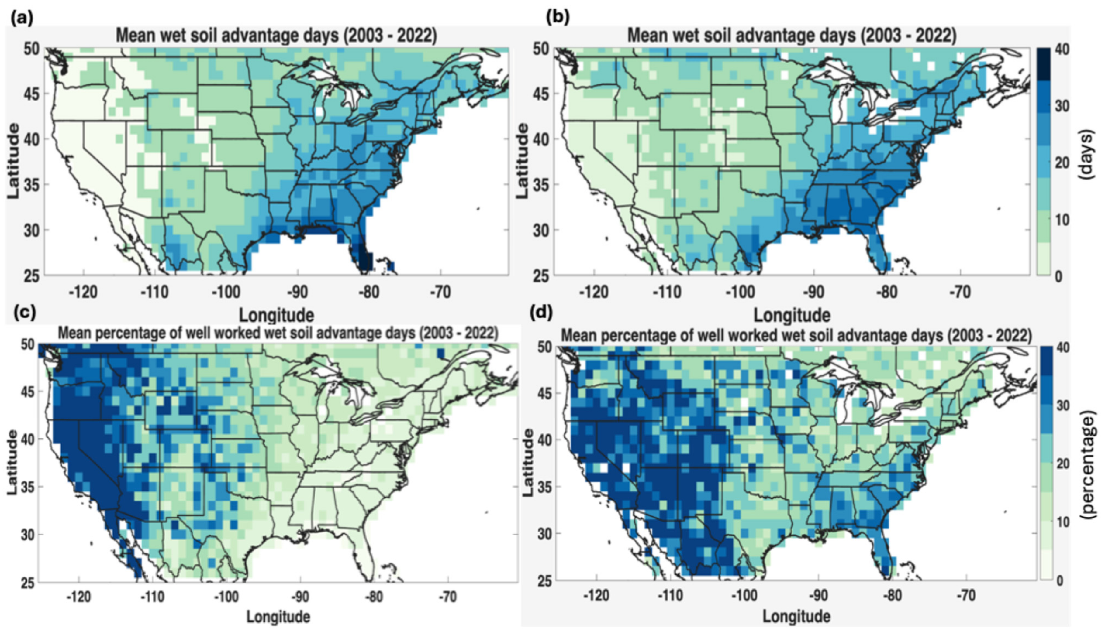
Wet soil advantage days for each year from 2003 to 2022, during the months of April to September, were calculated at each grid point and then averaged over this 20-year period. Two different results were obtained based on the use of ERA5 and NLDAS soil moisture and precipitation data, along with AIRS CTP-HIlow, for calculating wet and dry soil advantage days. Note that a greater number of wet soil advantage days are present in the eastern and southeastern part of the USA in both datasets, with the frequency being higher in the NLDAS case (Figure 4). These results are expected, since the eastern parts of the USA receive more precipitation [42].
Figure 4.
Spatial distribution of mean wet soil advantage days from 2003 to 2022 using (a) ERA5 and (b) NLDAS datasets; mean wet soil advantage hit percentage using (c) ERA5 and (d) NLDAS.
Then the wet soil hit percentage for each grid point was calculated for each year from 2003 to 2022 separately using Equation (3) and then averaged over the year using both ERA5 and NLDAS datasets. The wet hit percentage is greater over the western part of the country for both datasets. These days are more concentrated over the California, Nevada, and west Arizona regions in ERA5, while they are extended more towards the east and cover Colorado, New Mexico and west Texas regions in NLDAS datasets.
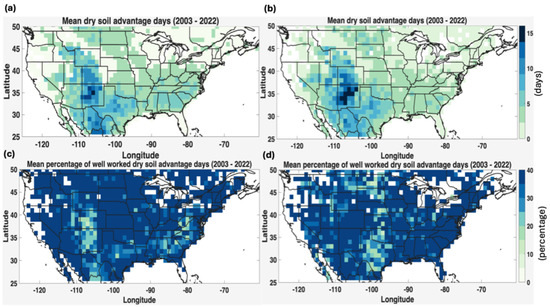
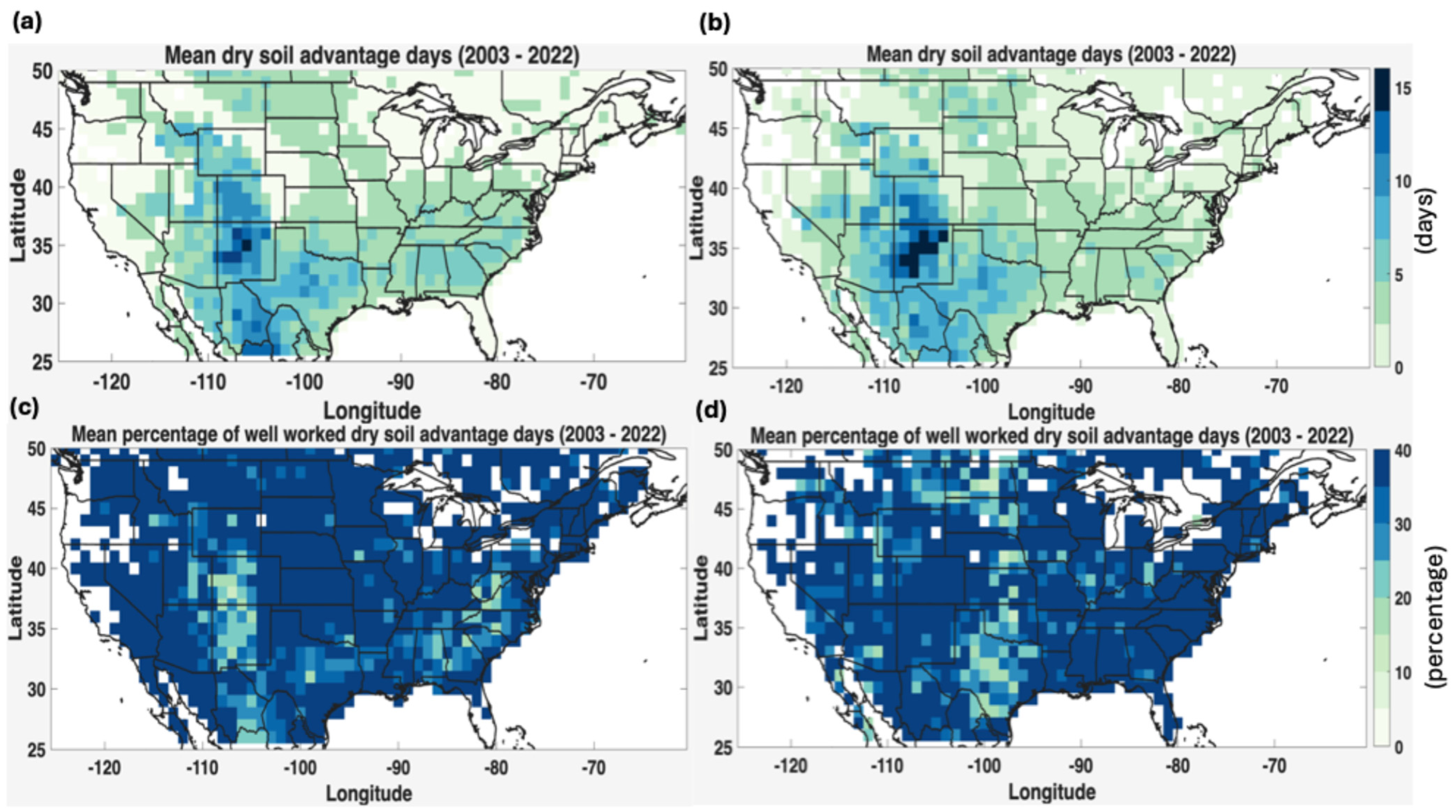
Similarly, dry soil advantage days for each year from 2003 to 2022 for April to September were calculated at each grid point and then averaged over the 20 years (Figure 5). Two different results based on the use of ERA5 and NLDAS soil moisture and precipitation data with AIRS CTP-HIlow for calculating wet and dry soil advantage days are presented. There are more dry soil advantage days over New Mexico and north Texas regions in both datasets. But the NLDAS data gives a greater number of dry soil advantage days over the New Mexico region compared to ERA5 data.
Figure 5.
Spatial distribution of mean dry soil advantage days from 2003 to 2022 using (a) ERA5 and (b) NLDAS datasets; mean dry soil advantage hit percentage using (c) ERA5 and (d) NLDAS.
Then, the frequency of dry soil hit percentage for each grid from both the datasets was calculated using Equation (4) (Figure 4c,d). The results indicate that dry soil advantage days are more distributed across the region. However, certain areas, such as New Mexico, Colorado, and Texas, are not well predicted either by the ERA5 or NLDAS datasets.
3.1.2. Climatology of Wet and Dry Soil Advantage Days at Four Selected North American Sites
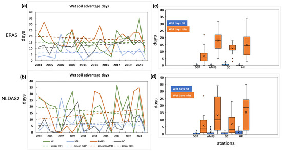
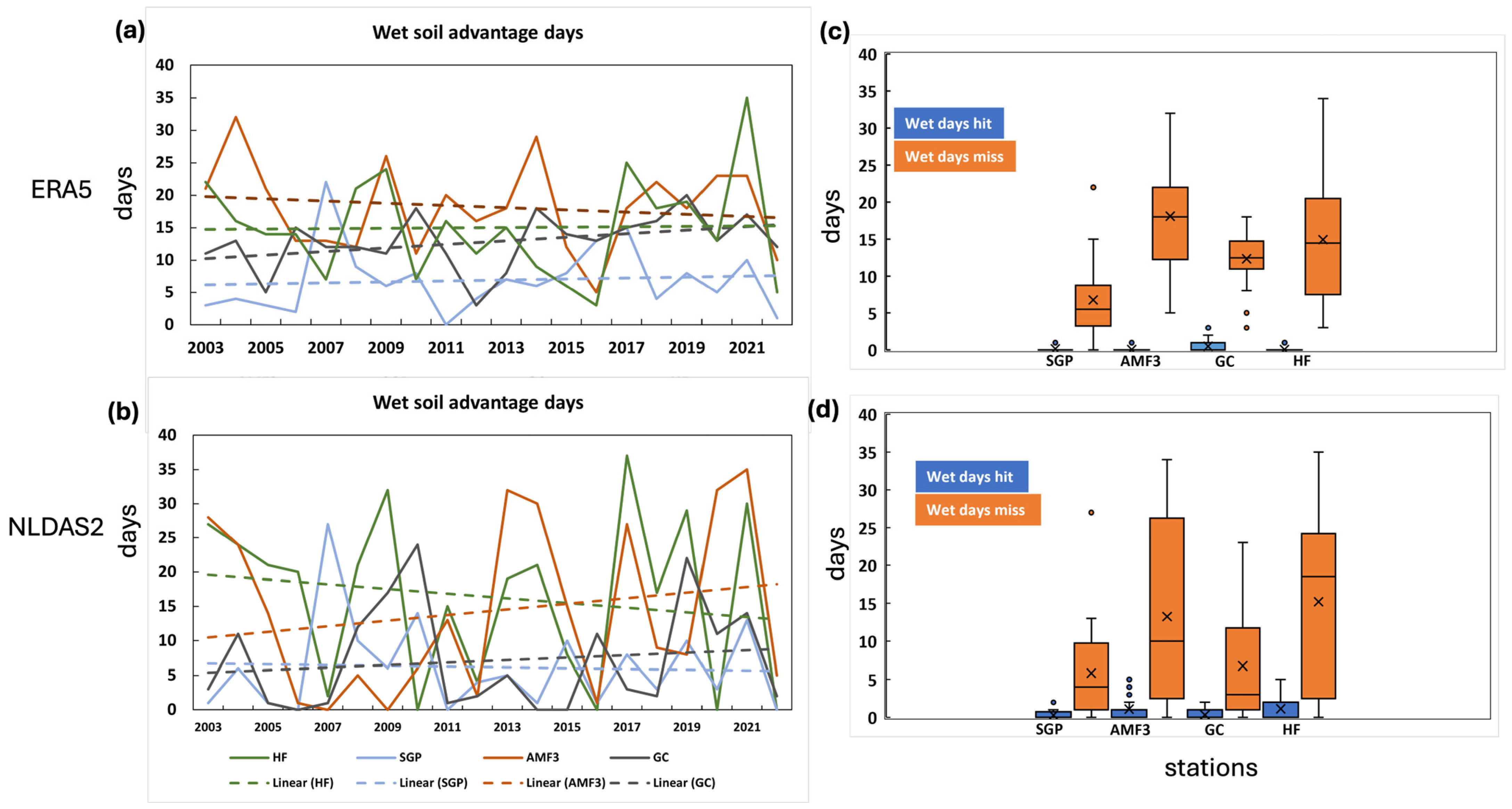
Interannual variation in wet soil advantage days over four previously mentioned sites (ARM-SGP, ARM-AMF3, Goodwater Creek (GC) and Harvard Forest (HF)) were calculated for each year (2003–2022) from ERA5 and NLDAS datasets and are presented in Figure 6a,b.
Figure 6.
Interannual variation in wet soil advantage days at ARM-SGP, ARM-AMF3, Goodwater Creek and Harvard Forest using (a) AIRS CTP-HI and ERA5 soil moisture and precipitation, (b) AIRS CTP-HI and NLDAS2 soil moisture and precipitation; box and whisker diagram for wet soil advantage hit and miss days using (c) AIRS CTP-HI and ERA5 soil moisture and precipitation, and (d) AIRS CTP-HI and NLDAS2 soil moisture and precipitation.
Within the ERA5 framework, the ARM-SGP and GC stations exhibit a higher wet soil advantage day annual event frequency, while the HF station maintains a relatively stationary baseline. NLDAS-2, by contrast, captures an opposing signal at these same locations showing negative deviations across both the SGP and HF domains over the same multi-decadal period. A similarly reversed pattern emerges at the ARM-AMF3 station. ERA5 indicates a long-term decline in event frequency, while NLDAS-2 shows a distinct shift toward higher events in recent years.
Box and whisker plots help quantify the hit and miss percentage for wet soil advantage days over each of the four stations for both datasets (Figure 6c,d). These show that wet day and dry day misses are more frequent over all four stations when compared to wet day and dry day hits from both datasets. Using ERA5 datasets, we observe that the wet day misses are most frequent at the AMF3 station followed by HF, GC, and SGP stations, but wet day hits are only present over station GC. Using NLDAS datasets, wet day misses are more numerous at the AMF3 station followed by HF, GC, and SGP stations, whereas wet day hits are more present at the HF station, a feature seen as almost the same at the other three stations.
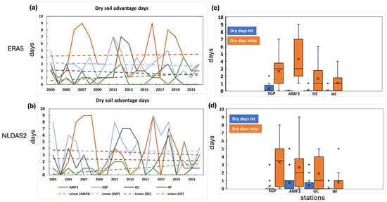
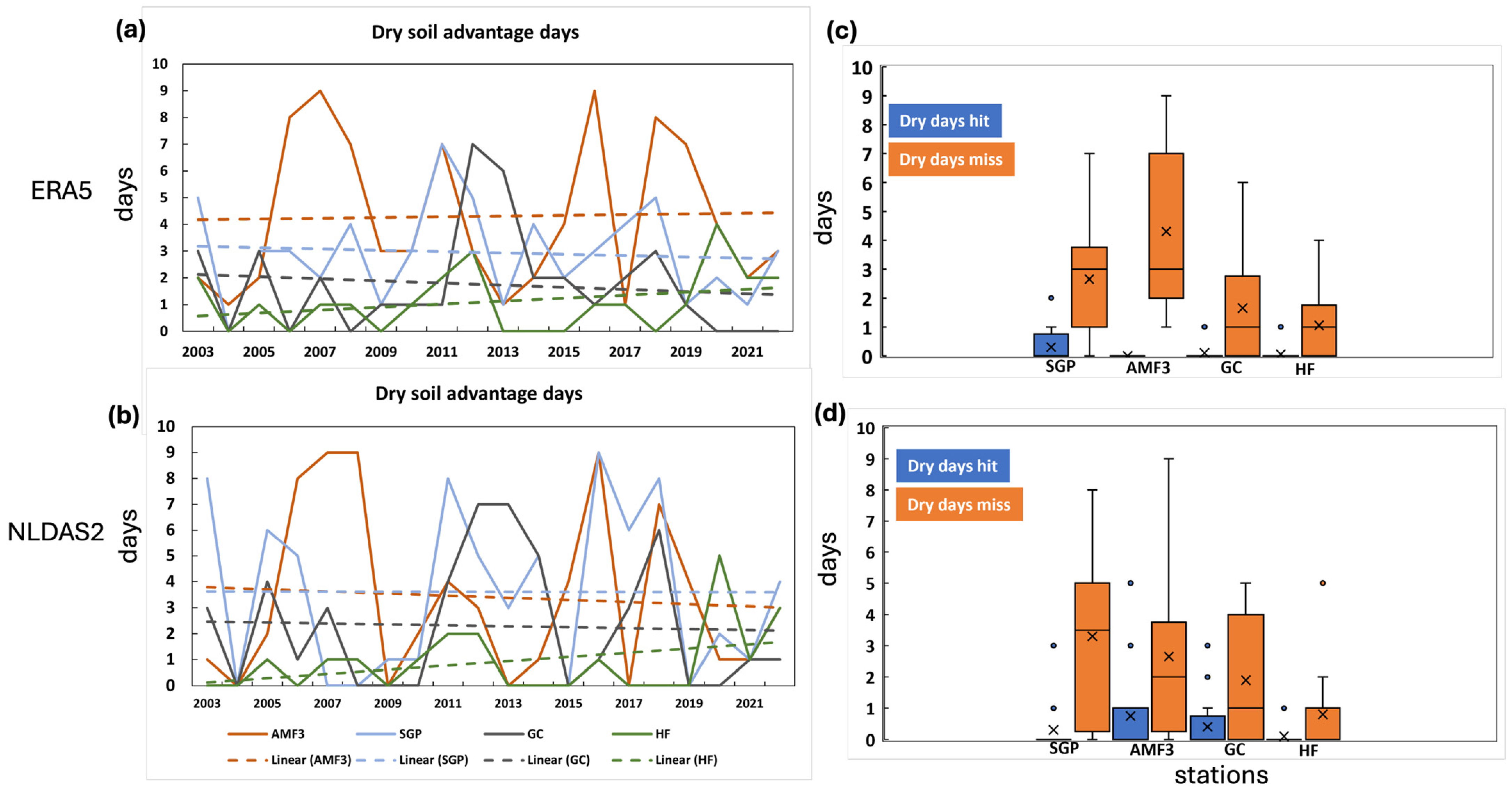
The interannual distribution of dry soil advantage days across the four stations similarly reveals spatially heterogeneous variability and systematic discrepancies between the ERA5 (Figure 7a) and NLDAS-2 (Figure 7b) reanalysis products over the 2003–2022 period. Within the ERA5 framework, annual event frequency is consistently higher at the ARM-AMF3 and HF stations, whereas the SGP and GC stations record markedly fewer days per year, suggesting a dipole-like spatial structure in reanalysis-derived soil moisture stress representation. The NLDAS-2 product yields a divergent regional distribution, with elevated day counts confined to the HF station and comparatively lower frequencies characterizing both the AMF3 and GC stations; the SGP station, by contrast, maintains a relatively stable and moderate annual count.
Figure 7.
Interannual variation in dry soil advantage days over ARM-SGP, ARM-AMF3, Goodwater Creek and Harvard Forest using (a) AIRS CTP-HI and ERA5 soil moisture and precipitation, (b) AIRS CTP-HI and NLDAS2 soil moisture and precipitation; box and whisker diagram for dry soil advantage hit and miss days using (c) AIRS CTP-HI and ERA5 soil moisture and precipitation, and (d) AIRS CTP-HI and NLDAS2 soil moisture and precipitation.
Box and whisker plots for dry day hit and miss days (Figure 7c,d) indicate that dry day misses are more present at AMF3, followed by the SGP, GC, and HF stations, and dry day hits are only present for the SGP station from ERA5 data. Using NLDAS2 data, dry day misses are more present at the SGP station, followed by the GC, AMF3 and HF stations. Dry day hits are more present at the AMF3 station followed by the GC station.
From both the above analyses, we find that there are several days at the stations having both wet soil and dry soil miss days. Periods with more than three consecutive wet soil and dry soil miss days during the 2003 to 2022 summer seasons were selected across the four stations shown in Table 1. There were no more than three consecutive dry soil miss days over HF, the Massachusetts station.
Consequently, for further large-scale analysis, wet soil and dry soil miss days at three stations (AMF3, SGP, and GC) have been considered and a detailed explanation is presented in the next section.
3.2. Large-Scale Meteorological Features for Wet Soil and Dry Soil Miss Periods
To investigate the reasons for the absence of afternoon precipitation on wet and dry soil advantage days, composite features of various meteorological parameters—including the horizontal moisture flux at the 850 hPa vertical level, pressure vertical velocity at 500 hPa, and vertical wind shear of horizontal wind (1000 hPa–700 hPa)—were analyzed for the period shown in Table 1.
The horizontal moisture flux magnitude at the 850 hPa pressure level was calculated using hourly specific humidity and horizontal wind components. At each grid point, the zonal () and meridional () components of the moisture transport are defined as:
where u is the zonal wind (ms−1), v is the meridional wind (ms−1), and q is the specific humidity (kg kg−1). The total horizontal moisture flux magnitude () plotted in the figures is subsequently derived as:
Given that this represents a single-level intensity rather than a vertically integrated column mass transport, the final field is expressed in units of kg kg−1 m s−1.
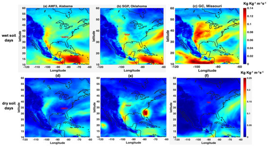
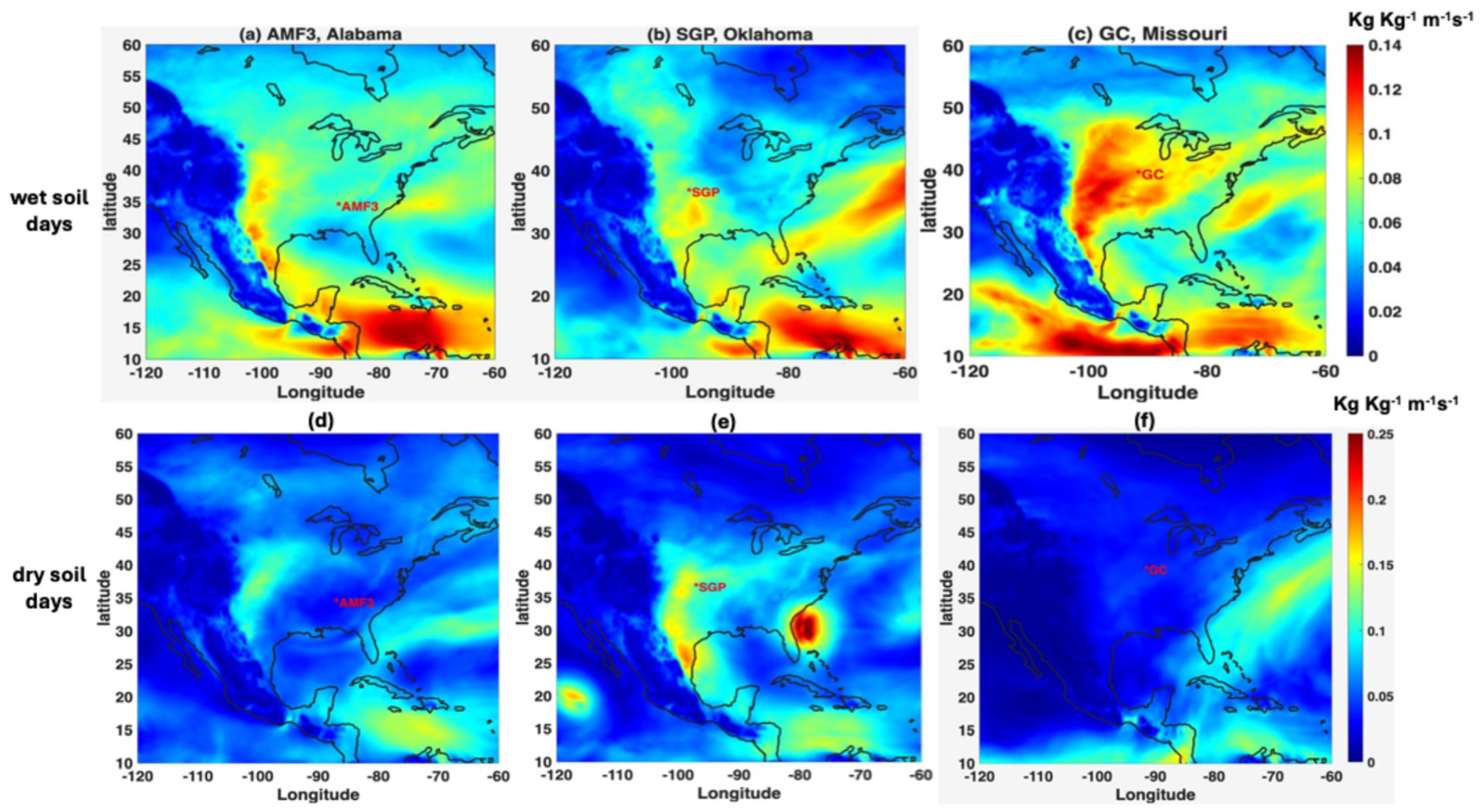
The spatial distribution of composite means of the 850 hPa moisture flux for wet soil miss periods at three locations (Figure 8a–c) reveals distinct differences between forested and agricultural plain regions. At the AMF3 station, Alabama, with forested land cover, a relatively moderate moisture flux pocket is observed in the western vicinity of the station. The forested surface, through higher evapotranspiration efficiency and canopy interception, contributes to a more spatially diffuse moisture transport pattern, with flux values appearing moderate but broadly distributed across the domain. In contrast, over the predominantly agricultural plain stations of SGP (Oklahoma) and GC (Missouri), the moisture flux is comparatively more concentrated and intense near the station locations, likely reflecting the role of large-scale low-level jet interactions with flat, agriculturally managed surfaces that offer lower aerodynamic resistance and more uniform moisture release.
Figure 8.
Composite mean of moisture flux at 850 hPa (kg/kg/m/s) for wet soil miss periods over (a) *AMF3, Alabama, (b) *SGP, Oklahoma, (c) *GC, Missouri; (d–f) same as (a–c) but for dry soil miss periods.
During dry soil miss days (Figure 8d–f), this contrast becomes even more pronounced. Over AMF3, the forested land surface sustains a relatively higher residual moisture flux compared to the agricultural plain stations, likely owing to the deeper root systems and higher soil water retention capacity characteristic of forested ecosystems. Conversely, over SGP and GC, moisture flux is substantially reduced during dry soil conditions, reflecting the greater sensitivity of agricultural plains to surface soil moisture deficits and their limited capacity to maintain atmospheric moisture supply under dry antecedent conditions. This reduction in moisture flux over the agricultural plains during dry soil miss days implies a stronger coupling between surface dryness and atmospheric moisture transport in these regions compared to forested areas. The contrast between forested and agricultural land surfaces in modulating moisture flux highlights the critical role of land cover type in mediating the soil moisture–atmosphere feedback, with forested regions exhibiting greater buffering capacity against surface moisture variability than agricultural plains.
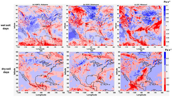
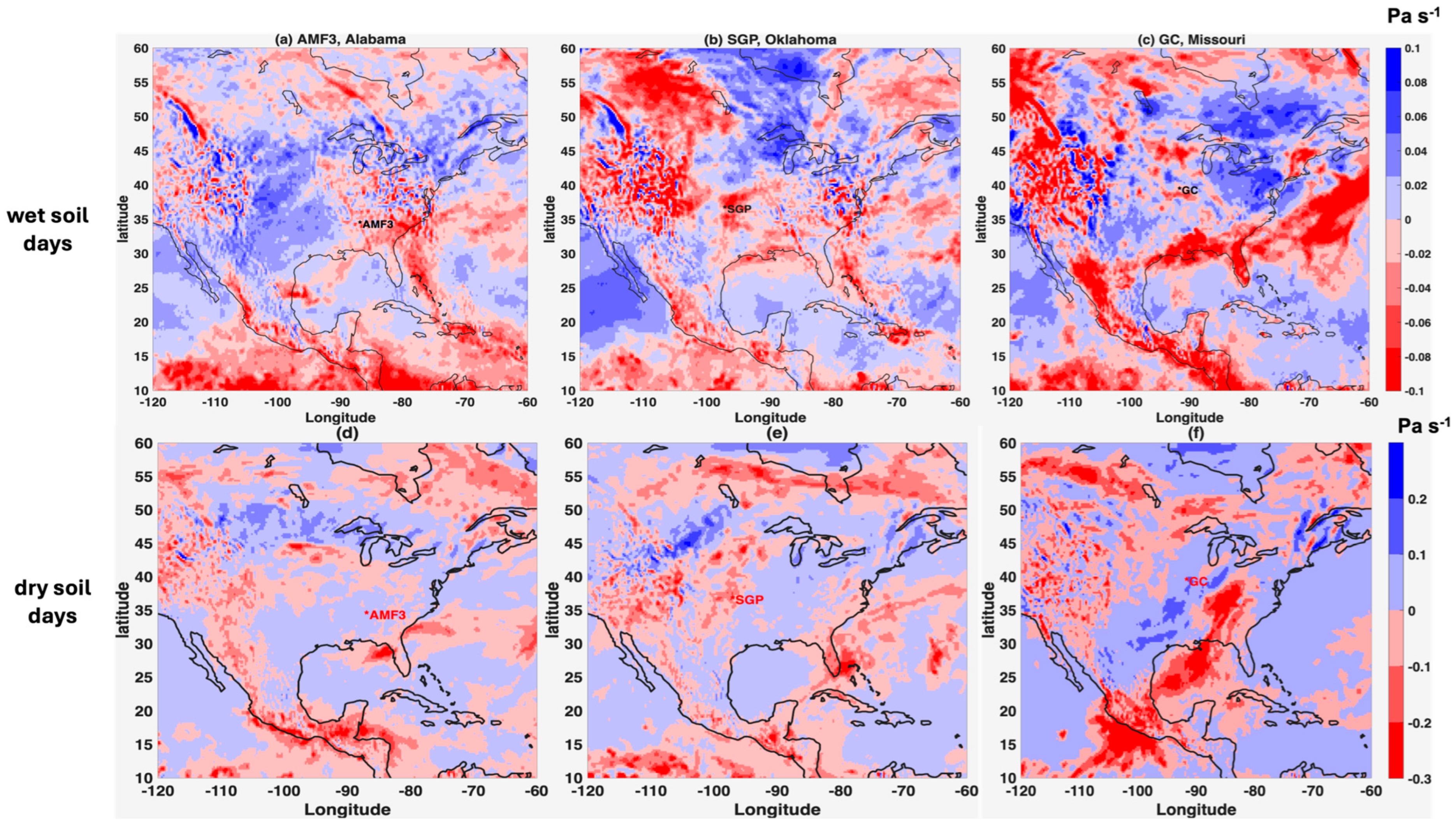
Further analysis of composite means of pressure vertical velocity (omega) at 500 hPa for all selected wet soil and dry soil advantage miss days over three stations (Figure 9a–f) shows rising motion over the station locations during the wet soil advantage miss period, which would support cloud formation and subsequent precipitation. In pressure coordinates negative omega generally means upward motion and positive omega means downward motion. In contrast, pressure vertical velocity indicates sinking motion during the dry soil advantage miss period, which is generally associated with drier conditions and suppressed convection. This reduction in moisture flux and the presence of downward motion implies a weaker connection between surface moisture and atmospheric processes, potentially affecting local weather patterns and precipitation.
Figure 9.
Composite mean of pressure vertical velocity at 500 hPa (Pa/s) for wet soil miss periods over (a) *AMF3, Alabama, (b) *SGP, Oklahoma, (c) *GC, Missouri; (d–f) same as (a–c) but for dry soil miss periods.
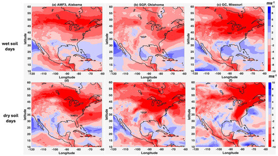
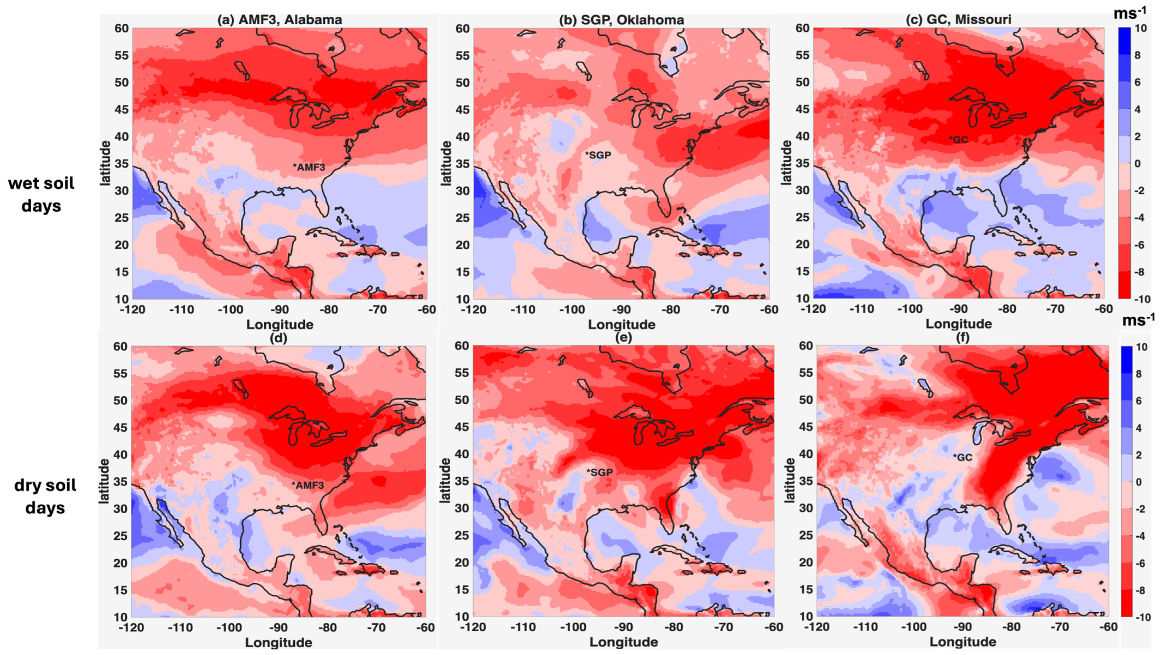
Furthermore, the composite means of vertical wind shear of horizontal wind between 1000 hPa and 700 hPa for all the events has been calculated and presented in Figure 10a–f. To ensure absolute mathematical and physical rigor, we have completely recalculated the diagnostic across all analysis figures to represent true vector bulk wind shear magnitude (), rather than a scalar speed difference.
where u and v represent the zonal and meridional wind components at 700 and 1000 hPa pressure levels. This represents the true vector bulk wind shear magnitude between the two pressure levels. By calculating the component-wise differences before computing the magnitude, this diagnostic better accounts for changes in both wind speed and wind direction (directional shear) within the column. Elevated vector shear magnitudes characterize a highly dynamic and turbulent vertical structure, which tilts or tears apart developing updrafts, thereby inhibiting the vertical development of convective clouds and suppressing precipitation at the station locations. Because a vector magnitude is inherently positive, a larger value directly signifies a more hostile dynamic environment for convective initiation.
Figure 10.
Composite mean of vertical wind shear (m/s) for wet soil miss periods over (a) *AMF3, Alabama, (b) *SGP, Oklahoma, (c) GC, Missouri; (d–f) same as (a–c) but for dry soil miss periods.
Figure 10 illustrates the spatial distribution of the true vector bulk wind shear magnitude between 1000 hPa and 700 hPa. A distinct, coherent band of enhanced vertical wind shear is observed across the northern sectors of all station domains. Near the three specific station locations (AMF3, SGP, and GC), the vector wind shear magnitudes during wet soil miss days are persistently high, ranging approximately from 2 to 4 ms−1. This kinematic suppression intensifies significantly during dry soil miss days, with local shear magnitudes swelling to between 4 and 6 ms−1. These elevated vector wind shear magnitudes create a hostile dynamic environment by tilting or venting emerging thermal plumes, which suppresses the vertical development of deep convective clouds and inhibits afternoon precipitation across the stations. This spatial pattern highlights how robust atmospheric dynamics can override favorable thermodynamic local surface coupling, regardless of underlying soil moisture conditions. In contrast, due to the absence of three consecutive wet and dry soil hit days, only single-day events were considered for comparison. Composite analysis for wet hit and dry hit days shows notably weaker wind shear magnitudes approximately from 2 to 3 ms−1. The comparatively weaker wind shear on hit days is dynamically consistent with a less hostile environment for convective initiation, allowing sufficient vertical development of clouds and enabling precipitation to occur at the station. This contrast between hit and miss days strongly suggests that vertical wind shear acts as a primary atmospheric control on convective precipitation, overriding the influence of antecedent soil moisture conditions. When wind shear is weak, atmospheric instability can be more readily released, facilitating precipitation regardless of soil moisture state, whereas strong wind shear during miss days effectively decouples the surface moisture signal from the overlying convective environment, suppressing rainfall.
To provide additional observational support for the wind shear suppression mechanism identified in the ERA5 composite analysis, we examined high-precision observations from the 915 MHz Radar Wind Profiler (RWP) consensus wind dataset (915rwpwindcon) at the ARM SGP site [43]. It should be noted, however, that continuous RWP data coinciding with the identified miss day periods were limited in availability due to instrument-related data gaps. The RWP analysis was therefore confined to the periods for which quality-controlled, continuous records exist, and the results should be interpreted as preliminary, limited-period observational support rather than as a comprehensive confirmation of the ERA5-derived findings. The RWP-derived mean vertical wind shear for wet miss and dry miss days was approximately 12.38 m s−1 and 12.33 m s−1, respectively, which is notably higher in magnitude than the ERA5 composite values of 2–6 m s−1. This discrepancy is attributed to fundamental differences in the nature of the two datasets: the ERA5 values represent spatially and temporally averaged composites across multiple miss day events on a coarse grid, which substantially smooths instantaneous shear magnitudes, whereas the RWP captures high-temporal-resolution point observations that reflect peak shear values during specific suppression episodes. Given these differences in spatial scale and temporal averaging, the two datasets are not directly numerically comparable but are instead treated as complementary lines of independent evidence, both consistently indicating the presence of anomalously strong vertical wind shear during miss day conditions.
We performed two-sample Student’s t-tests between wet soil miss and dry soil miss composites at each grid point. The results show that no grid cells exhibit statistically significant differences at the p < 0.05 level. This indicates that, within the limitations of the available sample size and variability, we do not find sufficient statistical evidence to distinguish the two composite regimes based on the examined wind shear fields. We therefore revise the interpretation to emphasize that the observed spatial structures represent qualitative and physically consistent patterns across the sampled cases, rather than statistically distinct mean states. We also acknowledge that the absence of statistical significance may reflect limited sample size and intrinsic atmospheric variability.
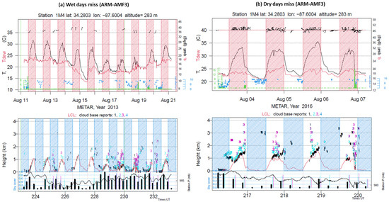
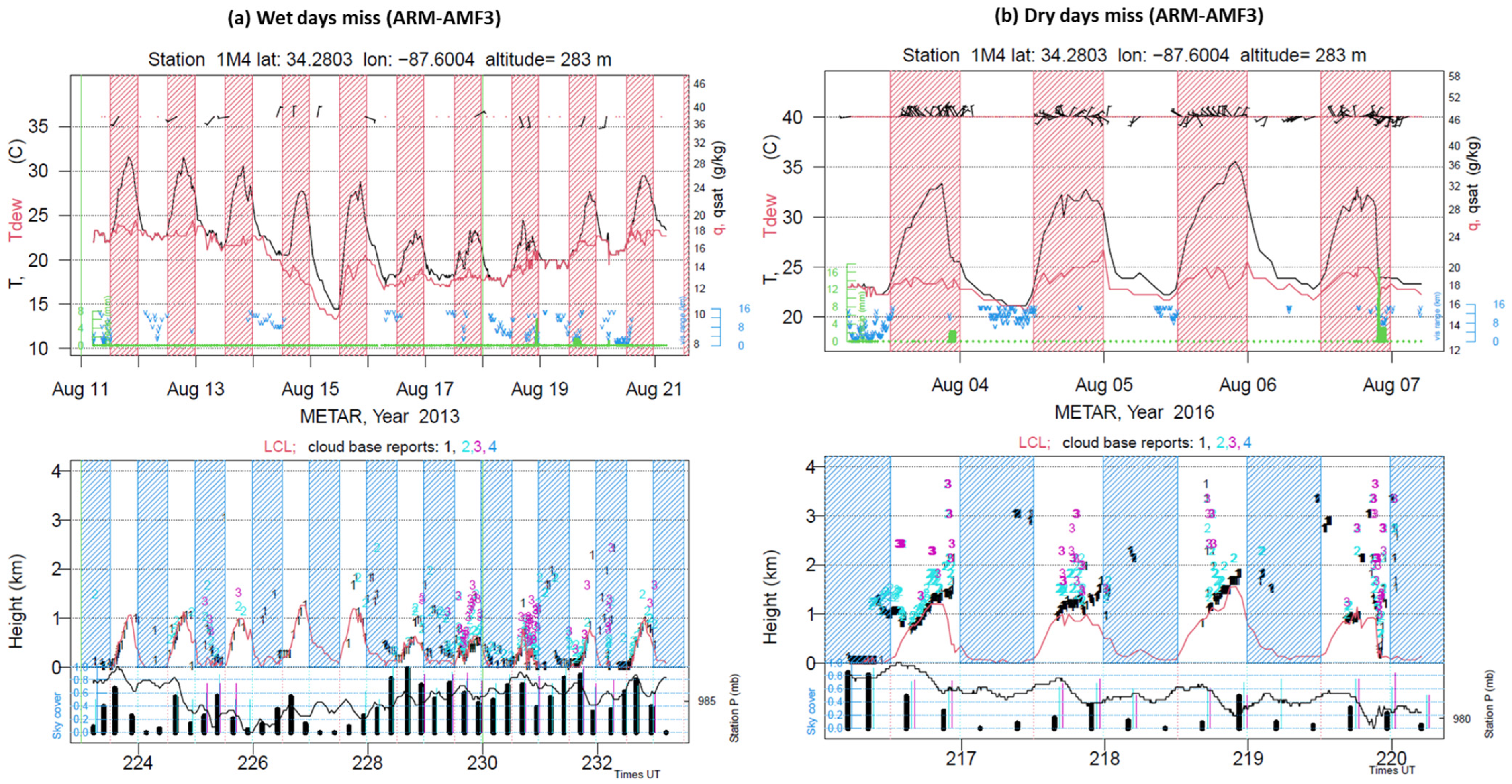
Additionally, analysis of lower-level meteorological features up to 4 km, using ASOS datasets, further supports these findings. One wet soil miss case, and one dry soil miss case over the AMF3 Alabama station were analyzed (Figure 11a,b). The results indicate that lower-level temperatures are lower on wet soil miss days compared to dry soil miss days. Stronger winds are observed during the nighttime for dry soil miss days, suggesting more stable conditions. Moreover, cloud fraction is higher on wet soil miss days compared to dry soil miss days, reinforcing the idea that increased soil moisture influences cloud cover but does not necessarily lead to precipitation due to the presence of strong wind shear.
Figure 11.
Sample comprehensive time series plots for two periods for METAR station K1M4, Haleyville Alabama, the closest station to AMF3. (Left) Period of 11–21 August 2013 (wet day misses), and (Right) 3–7 August 2016 (dry day misses). Each plot configured as follows. Top panel, top to bottom, hourly data: Wind barbs (10 m; in m/s); 2 m temperature (°C, black); 2 m dew point (°C, red); surface visual range (km, blue “v”); and liquid equivalent precipitation (mm, green). Red hatching shows effective ‘daytime’ period, one hour after astronomical ‘last sunrise’ to one hour before ‘first sunset’. Bottom panel: Top to bottom: Lifting condensation level (km, based on 2 m observations; red); ceilometer records of cloud base at up to four levels (“1”, “2”, “3”, “4”); where level “1” (black) represents the lowest detected cloud base, level “2” (cyan) the second lowest, level “3” (magenta/pink) the third, and level “4” (blue) the highest detected layer; lower section: Six-hourly cloud cover fraction (%), at each reporting level; hourly report of surface pressure (mb, black line). Blue hatching shows effective ’nocturnal’ period, the complement of the red hatching in the upper panel.
4. Conclusions
This study examined how well the CTP-HIlow framework does in predicting afternoon precipitation on wet and dry soil advantage days for selected stations. A comprehensive analysis of 20 years (2003–2022) of CTP-HIlow data over the CONUS during the summer season (April–September), utilizing remote sensing (AIRS), reanalysis datasets (ERA5, NLDAS2), and station observations (ASOS), provides valuable insights into soil moisture–atmosphere interactions. Our investigation of CTP-HIlow threshold values and afternoon rainfall across four flux net sites in North America, AMF3 (Alabama), SGP (Oklahoma), GC (Missouri), and HF (Massachusetts), further strengthens the findings.
A key conclusion is that the method has a geographical bias for success: wet soil advantage days are more frequent in the eastern and southeastern U.S., whereas the wet hit percentage is higher in the western region. Dry soil advantage days are predominant in New Mexico and northern Texas and serve as effective weather predictors, though certain areas, such as New Mexico, Colorado, and Texas, exhibit lower predictive accuracy. Additionally, multiple days experience both wet soil and dry soil miss conditions, in which meteorological indicators favor precipitation, yet none occurs. Composite analysis reveals persistently large wind shear magnitudes between 1000 hPa and 700 hPa during these miss days, ranging approximately from 4 to 6 m s−1, suggesting a dynamically unfavorable environment for deep convective development. While a direct causal link cannot be established from composite analysis alone, the systematic association between strong vertical wind shear and precipitation suppression on miss days points to atmospheric dynamics as a potentially important modulating factor, operating independently of antecedent soil moisture conditions. These findings highlight the need for future process-based investigations to more rigorously isolate the relative contributions of wind shear and surface moisture forcing to convective precipitation outcomes.
This study contributes new understanding of the CTP-HIlow framework by demonstrating its spatially varying predictive behavior across the CONUS using long-term satellite and reanalysis datasets. In contrast to earlier studies focused primarily on local or regional analyses, the present work reveals that the framework’s success strongly depends on regional atmospheric dynamics, particularly mid-level vertical wind shear. The identification of frequent wet and dry soil miss conditions despite favorable thermodynamic indicators highlights an important limitation of relying solely on early-morning land–atmosphere coupling metrics. Incorporating wind shear and other synoptic-scale controls therefore represents a significant advancement for improving convective precipitation forecasting.
Further studies should explore the interactions between synoptic-scale meteorological factors and the CTP-HIlow framework, including mid-level humidity, and mesoscale convective systems. Using high-resolution datasets, high-resolution numerical modeling and machine learning techniques can provide deeper insights into soil moisture–atmosphere feedback mechanisms. Additionally, expanding observational networks and refining threshold values for different climate regions will contribute to improving precipitation forecasting in complex weather conditions. Addressing these aspects will enhance predictive capabilities and support better decision-making in weather and climate studies.
Author Contributions
Conceptualization, D.R.F. and M.S.; methodology, D.R.F. and M.S.; validation, M.S.; writing—original draft preparation, M.S.; writing—review and editing, M.S.; visualization, M.S. All authors have read and agreed to the published version of the manuscript.
Funding
This research received no external funding.
Institutional Review Board Statement
Not applicable.
Informed Consent Statement
Not applicable.
Data Availability Statement
Data derived from public domain resources. The data presented in this study are available in: ASOS data: https://mesonet.agron.iastate.edu/request/download.phtml?network=AR__%20ASOS (accessed on 31 August 2023)”. AIRS data: https://disc.gsfc.nasa.gov/datasets?page=1&source=Aqua%20AIRS,Aqua%20AMSU-A,Aqua%20HSB&project=Aqua (accessed on 12 April 2023)”. ERA5 data: https://cds.climate.copernicus.eu/datasets/reanalysis-era5-single-levels?tab=download (accessed on 05 September 2023). NLDAS2 data: https://disc.gsfc.nasa.gov/datasets?keywords=NLDAS&page=1&subject=Precipitation (accessed on 10 September 2023).
Acknowledgments
This work has been supported by Craig R. Ferguson, National Aeronautics and Space Administration (when he was at the University at Albany). The authors are thankful to NASA, ECMWF, and Iowa State University for providing such valuable datasets. M.S. is grateful to the Atmospheric Science Research Center, University at Albany, for providing research infrastructure to carry out this work. The authors supplied funds for publishing this article.
Conflicts of Interest
The authors declare no conflicts of interest.
Abbreviations
The following abbreviations are used in this manuscript:
| CTP | convective triggering potential |
| HIlow | low-level humidity |
| AIRS | Atmospheric Infrared Sounder |
| CONUS | Continental United States |
| NLDAS-2 | North American Land Data Assimilation System |
| L-A | land–atmosphere |
| GEWEX | Global Energy and Water Exchanges |
| TCI | terrestrial coupling index |
| CBL | convective boundary layer |
| TP | Tibetan Plateau |
| WRF | Weather Research Forecast |
| PWP | Permanent Wilting Point |
| NCDC | National Climate Data Center |
| RMSE | root mean square error |
| ECMWF | European Center for Medium-Range Weather Forecasts |
| ASOS | Automated Surface Observing Systems |
| HF | Harvard Forest |
| SGP | Southern Great Plains |
| AMF3 | ARM Mobile Facility |
| GC | Goodwater Creek |
| METAR | METeorological Aerodrome Reports |
| LT | local time |
References
- Findell, K.L.; Eltahir, E.A. Atmospheric controls on soil moisture–boundary layer interactions. Part I: Framework development. J. Hydrometeorol. 2003, 4, 552–569. [Google Scholar] [CrossRef]
- Koster, R.D.; Sud, Y.C.; Guo, Z.; Dirmeyer, P.A.; Bonan, G.; Oleson, K.W.; Chan, E.; Verseghy, D.; Cox, P.; Davies, H.; et al. GLACE: The global land–atmosphere coupling experiment. Part I: Overview. J. Hydrometeorol. 2006, 7, 590–610. [Google Scholar] [CrossRef]
- Betts, A.K. Land-surface-atmosphere coupling in observations and models. J. Adv. Model. Earth Syst. 2009, 1, 4. [Google Scholar] [CrossRef]
- Zheng, Y.; Kumar, A.; Niyogi, D. Impacts of land–atmosphere coupling on regional rainfall and convection. Clim. Dyn. 2015, 44, 2383–2409. [Google Scholar] [CrossRef]
- Schumacher, D.L.; Keune, J.; Van Heerwaarden, C.C.; Vilà-Guerau de Arellano, J.; Teuling, A.J.; Miralles, D.G. Amplification of mega-heatwaves through heat torrents fuelled by upwind drought. Nat. Geosci. 2019, 12, 712–717. [Google Scholar] [CrossRef]
- Van Heerwaarden, C.C.; Teuling, A.J. Disentangling the response of forest and grassland energy exchange to heatwaves under idealized land–atmosphere coupling. Biogeosciences 2014, 11, 6159–6171. [Google Scholar] [CrossRef]
- Miralles, D.G.; Gentine, P.; Seneviratne, S.I.; Teuling, A.J. Land–atmospheric feedbacks during droughts and heatwaves: State of the science and current challenges. Ann. N. Y. Acad. Sci. 2019, 1436, 19–35. [Google Scholar] [CrossRef] [PubMed]
- Sud, Y.C.; Mocko, D.M.; Lau, K.M.; Atlas, R. Simulating the Midwestern US drought of 1988 with a GCM. J. Clim. 2003, 16, 3946–3965. [Google Scholar] [CrossRef]
- Laguë, M.M.; Bonan, G.B.; Swann, A.L. Separating the impact of individual land surface properties on the terrestrial surface energy budget in both the coupled and uncoupled land–atmosphere system. J. Clim. 2019, 32, 5725–5744. [Google Scholar] [CrossRef]
- Douville, H. Influence of soil moisture on the Asian and African monsoons. Part II: Interannual variability. J. Clim. 2002, 15, 701–720. [Google Scholar] [CrossRef]
- Betts, A.K.; Ball, J.H.; Beljaars, A.C.; Miller, M.J.; Viterbo, P.A. The land surface–atmosphere interaction: A review based on observational and global modeling perspectives. J. Geophys. Res. Atmos. 1996, 101, 7209–7225. [Google Scholar] [CrossRef]
- Betts, A.K.; Silva Dias, M.A.F. Progress in understanding land–surface–atmosphere coupling from LBA research. J. Adv. Model. Earth Syst. 2010, 2, 6. [Google Scholar] [CrossRef]
- Santanello, J.A., Jr.; Lawston, P.; Kumar, S.; Dennis, E. Understanding the impacts of soil moisture initial conditions on NWP in the context of land–atmosphere coupling. J. Hydrometeorol. 2019, 20, 793–819. [Google Scholar] [CrossRef]
- Delworth, T.L.; Manabe, S. The influence of potential evaporation on the variabilities of simulated soil wetness and climate. J. Clim. 1988, 1, 523–547. [Google Scholar] [CrossRef]
- Findell, K.L.; Eltahir, E.A. Atmospheric controls on soil moisture–boundary layer interactions. Part II: Feedbacks within the continental United States. J. Hydrometeorol. 2003, 4, 570–583. [Google Scholar] [CrossRef]
- Ferguson, C.R.; Wood, E.F. Observed land–atmosphere coupling from satellite remote sensing and reanalysis. J. Hydrometeorol. 2011, 12, 1221–1254. [Google Scholar] [CrossRef]
- Roundy, J.K.; Santanello, J.A. Utility of satellite remote sensing for land–atmosphere coupling and drought metrics. J. Hydrometeorol. 2017, 18, 863–877. [Google Scholar] [CrossRef] [PubMed]
- Ford, T.W.; Steiner, J.; Mason, B.; Quiring, S.M. Observation-Driven Characterization of Soil Moisture-Precipitation Interactions in the central United States. J. Geophys. Res. Atmos. 2023, 128, e2022JD037934. [Google Scholar] [CrossRef]
- Zhao, C.; Meng, X.; Li, Y.; Lyu, S.; Guo, J.; Liu, H. Impact of soil moisture on afternoon convection triggering over the Tibetan Plateau based on 1-D boundary layer model. J. Geophys. Res. Atmos. 2022, 127, e2021JD035591. [Google Scholar] [CrossRef]
- Roundy, J.K.; Ferguson, C.R.; Wood, E.F. Temporal variability of land–atmosphere coupling and its implications for drought over the southeast United States. J. Hydrometeorol. 2013, 14, 622–635. [Google Scholar] [CrossRef]
- Findell, K.L.; Gentine, P.; Lintner, B.R.; Kerr, C. Probability of afternoon precipitation in eastern United States and Mexico enhanced by high evaporation. Nat. Geosci. 2011, 4, 434–439. [Google Scholar] [CrossRef]
- Berg, A.; Findell, K.; Lintner, B.R.; Gentine, P.; Kerr, C. Precipitation sensitivity to surface heat fluxes over North America in reanalysis and model data. J. Hydrometeorol. 2013, 14, 722–743. [Google Scholar] [CrossRef]
- Findell, K.L.; Eltahir, E.A. Atmospheric controls on soil moisture–boundary layer interactions: Three-dimensional wind effects. J. Geophys. Res. Atmos. 2003, 108, 8385. [Google Scholar] [CrossRef]
- Ford, T.W.; Quiring, S.M.; Thakur, B.; Jogineedi, R.; Houston, A.; Yuan, S.; Kalra, A.; Lock, N. Evaluating soil moisture–precipitation interactions using remote sensing: A sensitivity analysis. J. Hydrometeorol. 2018, 19, 1237–1253. [Google Scholar] [CrossRef]
- Ford, T.W.; Rapp, A.D.; Quiring, S.M.; Blake, J. Soil moisture–precipitation coupling: Observations from the Oklahoma Mesonet and underlying physical mechanisms. Hydrol. Earth Syst. Sci. 2015, 19, 3617–3631. [Google Scholar] [CrossRef]
- Chen, L.; Dirmeyer, P.A.; Tawfik, A.; Lawrence, D.M. Sensitivities of land cover–precipitation feedback to convective triggering. J. Hydrometeorol. 2017, 18, 2265–2283. [Google Scholar] [CrossRef]
- Sun, J.; Pritchard, M.S. Effects of Explicit Convection on Land Surface Air Temperature and Land-Atmosphere Coupling in the Thermal Feedback Pathway. J. Adv. Model. Earth Syst. 2018, 10, 2376–2392. [Google Scholar] [CrossRef]
- Jach, L.; Warrach-Sagi, K.; Ingwersen, J.; Kaas, E.; Wulfmeyer, V. Land cover impacts on land-atmosphere coupling strength in climate simulations with WRF over Europe. J. Geophys. Res. Atmos. 2020, 125, e2019JD031989. [Google Scholar] [CrossRef]
- Kim, S.; Kumar, M.; Kam, J. Rain-fed to irrigation-fed transition of agriculture exacerbates meteorological drought in cropped regions but moderates elsewhere. Environ. Res. Lett. 2023, 18, 074024. [Google Scholar] [CrossRef]
- Cheng, W.Y.; Cotton, W.R. Sensitivity of a cloud-resolving simulation of the genesis of a mesoscale convective system to horizontal heterogeneities in soil moisture initialization. J. Hydrometeorol. 2004, 5, 934–958. [Google Scholar] [CrossRef]
- Drager, A.J.; Grant, L.D.; van den Heever, S.C. A Nonmonotonic Precipitation Response to Changes in Soil Moisture in the Presence of Vegetation. J. Hydrometeorol. 2022, 23, 1095–1111. [Google Scholar] [CrossRef]
- Meyer, C.I.; Ern, M.; Hoffmann, L.; Trinh, Q.T.; Alexander, M.J. Intercomparison of AIRS and HIRDLS stratospheric gravity wave observations. Atmos. Meas. Tech. 2018, 11, 215–232. [Google Scholar] [CrossRef]
- Tian, B.; Manning, E.; Roman, J.; Thrastarson, H.; Fetzer, E.; Monarrez, R. AIRS Version 7 Level 3 Product User Guide; Jet Propulsion Laboratory, California Institute of Technology: La Canada Flt, CA, USA, 2020. Available online: https://airs.jpl.nasa.gov/data/products/v7-L2-L3/ (accessed on 12 April 2023).
- Kahn, B.H.; Irion, F.W.; Dang, V.T.; Manning, E.M.; Nasiri, S.L.; Naud, C.M.; Blaisdell, J.M.; Schreier, M.M.; Yue, Q.; Bowman, K.W.; et al. The atmospheric infrared sounder version 6 cloud products. Atmos. Chem. Phys. 2014, 14, 399–426. [Google Scholar] [CrossRef]
- Ferguson, C.R.; Wood, E.F. An evaluation of satellite remote sensing data products for land surface hydrology: Atmospheric infrared sounder. J. Hydrometeorol. 2010, 11, 1234–1262. [Google Scholar] [CrossRef]
- Hoffmann, L.; Günther, G.; Li, D.; Stein, O.; Wu, X.; Griessbach, S.; Heng, Y.; Konopka, P.; Müller, R.; Vogel, B.; et al. From ERA-Interim to ERA5: The considerable impact of ECMWF’s next-generation reanalysis on Lagrangian transport simulations. Atmos. Chem. Phys. 2019, 19, 3097–3124. [Google Scholar] [CrossRef]
- Vogel, B.; Günther, G.; Müller, R.; Grooß, J.U.; Afchine, A.; Bozem, H.; Hoor, P.; Krämer, M.; Müller, S.; Riese, M.; et al. Long-range transport pathways of tropospheric source gases originating in Asia into the northern lower stratosphere during the Asian monsoon season 2012. Atmos. Chem. Phys. 2016, 16, 15301–15325. [Google Scholar] [CrossRef]
- Konopka, P.; Steinhorst, H.M.; Grooß, J.U.; Günther, G.; Müller, R.; Elkins, J.W.; Jost, H.J.; Richard, E.; Schmidt, U.; Toon, G.; et al. Mixing and ozone loss in the 1999–2000 Arctic vortex: Simulations with the three-dimensional Chemical Lagrangian Model of the Stratosphere (CLaMS). J. Geophys. Res. Atmos. 2004, 109, D02315. [Google Scholar] [CrossRef]
- FAA. Surface Weather Observing. FAA Order 7900.5E. 2020. Available online: http://www.faa.gov/regulations_policies/orders_notices (accessed on 31 August 2023).
- Landolt, S.D.; Gaydos, A.; Porter, D.; DiVito, S.; Jacobson, D.; Schwartz, A.J.; Thompson, G.; Lave, J. Inferring the presence of freezing drizzle using archived data from the Automated Surface Observing System (ASOS). J. Atmos. Ocean. Technol. 2020, 37, 2239–2250. [Google Scholar] [CrossRef]
- Gautam, S.; Costello, C.; Baffaut, C.; Thompson, A.; Svoma, B.M.; Phung, Q.A.; Sadler, E.J. Assessing long-term hydrological impact of climate change using an ensemble approach and comparison with global gridded model-a case study on Goodwater Creek Experimental Watershed. Water 2018, 10, 564. [Google Scholar] [CrossRef]
- Bartels, R.J.; Black, A.W.; Keim, B.D. Trends in precipitation days in the United States. Int. J. Climatol. 2020, 40, 1038–1048. [Google Scholar] [CrossRef]
- Atmospheric Radiation Measurement (ARM) User Facility. Radar Wind Profiler (915RWPWINDCON), 2007-06-21 to 2007-06-30, Southern Great Plains (SGP) Central Facility, Lamont, OK (C1); Coulter, R., Muradyan, P., Martin, T., Eds.; ARM Data Center: Oak Ridge, TN, USA, 1998. [Google Scholar] [CrossRef]

Disclaimer/Publisher’s Note: The statements, opinions and data contained in all publications are solely those of the individual author(s) and contributor(s) and not of MDPI and/or the editor(s). MDPI and/or the editor(s) disclaim responsibility for any injury to people or property resulting from any ideas, methods, instructions or products referred to in the content. |
© 2026 by the authors. Licensee MDPI, Basel, Switzerland. This article is an open access article distributed under the terms and conditions of the Creative Commons Attribution (CC BY) license.