


Abstract
This study investigates the forecast bust of Typhoon SHANSHAN (2024) characterized by large track errors using the four major interactive grand global operational ensemble data and the atmospheric reanalysis data. Ensemble space empirical orthogonal function (EOF) analysis is applied to 850, 500, and 300 hPa geopotential heights at three target times to diagnose how synoptic-scale uncertainty contributed to the erroneous motions of SHANSHAN. We align the multi-level EOF bases to a reference-time basis via a weighted Procrustes rotation and evaluate similarity to the atmospheric reanalysis data in the aligned principal component (PC) space, enabling robust, distance-based conditioning of ensemble members. Results show that ensemble spread is consistently larger in the mid-latitudes, with relatively large uncertainty concentrated around the upper-tropospheric trough and lower-tropospheric structure near SHANSHAN. The dominant EOF modes differ by phase of SHANSHAN: lower-tropospheric modes govern the westward-moving stage, whereas mid- and upper-tropospheric modes dominate after recurvature. Selecting members whose EOF-based PC structures most closely match the atmospheric reanalysis effectively suppresses large-error outliers and yields improved conditional track predictions. These findings highlight phase-dependent synoptic controls and demonstrate that adaptive, reference-consistent conditioning can enhance the track guidance of tropical cyclones during difficult forecast situations.
1. Introduction
Tropical cyclones (TCs) are among those natural phenomena on Earth that have a significant social and economic impact. The Observing System Research and Predictability Experiment (THORPEX) Interactive Grand Global Ensemble (TIGGE) [1] provides global ensemble forecast information computed by ensemble prediction systems operated at major numerical weather prediction (NWP) centers worldwide, and these ensemble products are widely used for TC track prediction. With advances in science and technology, the accuracy of TC track forecasts is improving but “forecast busts” or “dropouts”, that is, very large forecast track errors, still occur [2,3].
To understand the characteristics of TC tracks predicted by an ensemble prediction system and improve the ensemble system, the characteristics of the synoptic-scale environment on a weather-forecasting timescale should be explored. A common approach to objectively summarize dominant spatial structures in the synoptic-scale environment is principal component analysis (PCA), often referred to as empirical orthogonal function (EOF) analysis in meteorology. EOF analysis decomposes the variance of a field into orthogonal spatial modes, and its statistical interpretation can be introduced by concepts such as the effective spatial degrees of freedom (ESDOF) [4].
While EOF analysis has traditionally been applied to time-varying datasets (samples = time), the formulation is general and can be applied to any collection of spatial fields. By treating ensemble members or a set of models as samples, EOF analysis can be used to summarize inter-model variance and the structure of ensemble uncertainty; indeed, Coupled Model Intercomparison Project (CMIP) multi-model outputs have been compared and evaluated using leading EOF modes and related approaches [5,6]. Moreover, interpreting a multi-model “ensemble of opportunity” requires an explicit statistical framework, including the notion of reliability [7]. From this perspective, it is natural to go beyond the ensemble mean and ask what the internal structure of ensemble spread implies for forecast busts, namely, when and how the predicted synoptic environments diverge, and whether the divergence can be exploited to improve TC track predictions.
Motivated by the above perspective, by using TIGGE global ensemble data and the fifth-generation European Centre for Medium-Range Weather Forecasts (ECMWF) atmospheric reanalysis (ERA5) dataset [8], this study revisits the notable track-forecast bust of Typhoon SHANSHAN (2024) as a single-case synoptic diagnosis, focusing on the structure of ensemble uncertainty and its potential implications for its track prediction. The Regional Specialized Meteorological Center (RSMC)-Tokyo named SHANSHAN at 18 UTC on 21 August 2024, when the storm was located at 16.6° N, 142.2° E. SHANSHAN moved northward with slow intensification before turning northwestward and moving along a counterclockwise circulation of an upper cold low that had been cut off from an upper-tropospheric trough. SHANSHAN reached its peak intensity during this northwestward movement over a relatively warm ocean [9]. After recurvature back toward the north, the storm made landfall in Kyushu, Japan. Subsequently, it turned east and reverted to a tropical depression, despite its mid-latitude location. SHANSHAN’s movement was therefore related both to its intensity and the characteristics of synoptic-scale environment, particularly in the mid-latitudes. This study focuses on SHANSHAN’s track errors rather than the intensity change and examines the synoptic-scale uncertainty structure underlying those errors.
The central scientific questions are as follows: (1) When the track predictions of SHANSHAN failed, which synoptic elements (e.g., mid-latitude troughs, upper-level cold lows, and the flow along the subtropical high) exhibited the largest ensemble uncertainty and how did that uncertainty project onto the track errors? (2) Even when the ensemble mean fails, can the track prediction be improved by identifying and conditioning on ensemble members whose synoptic environments are more consistent with a reference reanalysis such as ERA5? To address these questions, we set the following objectives:
(a) To clarify the mathematical basis of ensemble EOF analysis. We emphasize that EOF/PCA is fundamentally a variance decomposition over a sample set. We also present a concise framework for interpreting ensemble EOFs (including standardization, sign alignment, mode interpretation, weighted Procrustes rotation, and similarity metrics).
(b) To extract the structure of synoptic-scale diversity (ensemble spread). We construct a grand ensemble dataset combining TIGGE multi-center ensembles and ERA5 as a reanalysis reference and objectively describe how synoptic-scale spread manifests as dominant EOF patterns at the targeted times.
(c) To re-evaluate the relationship between synoptic environments and the track of SHANSHAN. We examine how the leading EOF modes and associated normalized amplitudes relate to track errors, providing a single-case demonstration of how synoptic uncertainty projects onto the track predictions.
(d) To discuss the potential for improvement of SHANSHAN’s track predictions via conditioning on reanalysis-consistent members. Rather than relying solely on the ensemble mean, we evaluate whether selecting a subset of members with synoptic environments most similar to the reanalysis can yield improved track estimates, while explicitly acknowledging the limitations of inference from a single event.
The rest of this paper is constructed as follows. Section 2 summarizes the ensemble space EOF framework used to diagnose synoptic-scale uncertainty. Section 3 describes the datasets and pre-processing—TIGGE multi-center forecasts and the ERA5 reanalysis—together with the alignment and selection procedures. Section 4 presents the results at three target times that bracket the westward-moving and post-landfall phases, including level-/mode-wise contributions, a synoptic interpretation, and the linkage between mode reproducibility and track position error. Section 5 discusses implications, limitations, and future directions. Section 6 is devoted to the conclusion.
2. Mathematical Background
EOF analysis is mathematically equivalent to PCA and provides an objective method for extracting dominant patterns of variability from a set of spatial fields. In this study, EOF analysis is applied not to a time-series but to an ensemble of NWP fields. This section summarizes the mathematical foundation of EOF analysis and clarifies how it is adapted for use in ensemble space.
2.1. Principal Component Analysis (PCA)
Let M be the number of grid points (after masking/area weighting) and N the number of samples (ensemble members). Construct X ∈ ℝ^{M × N} whose i-th column is the anomaly field vector xi (optionally standardized; see Section 2.4). The sample covariance in “space” is C; EOF modes are eigenvectors of C. When M ≫ N, C is rank ≤ N − 1 and it is computationally efficient to solve the equivalent eigenproblem for (dimension N × N) and map back to spatial EOFs.
Let
be a data matrix whose columns represent N samples of a spatial field with dimension M. The sample covariance matrix is defined as
EOF analysis seeks the eigenvectors ek and eigenvalues λk that satisfy
The eigenvectors ek represent orthogonal spatial patterns, and the associated principal component (PC) coefficients are given by
The eigenvalue λk corresponds to the variance explained by the k-th mode and the fractional variance contribution is
2.2. Time-Series EOF vs. Ensemble EOF
EOF analysis has traditionally been used to extract dominant modes of variability from time-varying atmospheric fields. In such applications, the samples xi correspond to different times, and the PCs represent temporal evolution. However, the mathematical formulation does not require the samples to be time-ordered. Any collection of spatial fields can be analyzed, provided they are defined on a common grid and represent realizations of a common physical system. Two complementary distinctions clarify “time-series EOF” vs. “ensemble EOF”:
- (i)
- Mathematical:
The sample index i labels the columns of X, representing either time or ensemble members, and the eigenproblem is the same in both cases.
- (ii)
- Conceptual:
In time-series EOF, leading modes summarize temporal variability; in ensemble EOF, leading modes summarize the spatial structure of forecast uncertainty (ensemble spread) at a fixed target time. In this study, the samples xi correspond to different ensemble members rather than different times. Thus, the analysis is performed in ensemble space, where variability reflects differences among NWP models, initial conditions, and forecast lead times (FT). This interpretation is consistent with the ensemble synoptic analysis framework, which treats probabilistic samples at one or more instants in time as a valid basis to diagnose spatial relationships [10].
Mathematically, the formulation is identical to time-series EOF analysis. The distinction lies in the interpretation:
- -
- Time-series EOF: Dominant modes of temporal variability.
- -
- Ensemble EOF: Dominant modes of ensemble spread (uncertainty structure).
This distinction is essential for understanding the purpose of the present study. Ensemble EOFs identify the spatial patterns along which the ensemble members differ most strongly, thereby revealing the structure of forecast uncertainty.
2.3. Physical Interpretation of Ensemble EOF Modes
This subsection notes the following on sample size: In synoptic applications, the grid dimension M is typically much larger than the ensemble size N. Hence, only up to N − 1 independent EOF modes can be estimated, and higher-order modes may be sensitive to sampling noise. This motivates focusing on leading modes and reporting the cumulative explained variance and robustness diagnostics. The leading EOF modes represent the principal directions of ensemble spread. For each mode k, the PC coefficient ak,i indicates how strongly the i-th ensemble member projects onto the spatial pattern ek.
The variance of the PC coefficients is
so the first EOF mode (EOF1) corresponds to the direction of maximum ensemble variance.
In the context of TC prediction, these modes often reflect the following synoptic features, for example:
- -
- Differences in the position or amplitude of mid-latitude troughs;
- -
- Variations in the strength or extent of the subtropical high;
- -
- Differences in upper-level steering flow and mid-latitude jet streaks;
- -
- Structural differences in the synoptic environment.
Thus, ensemble EOFs provide a compact representation of the synoptic-scale uncertainty that influences TC track predictions.
2.4. Standardization and Sign Alignment
Standardization in “ensemble space”: For each grid point m, compute the ensemble mean μm and standard deviation σm across members at the same target time. Each anomaly is formed as . If standardized EOFs are used, define (with σm > 0; grid points with near-zero σm are masked). This yields a correlation-type EOF that emphasizes relative spread rather than absolute units. If unstandardized EOFs are used, EOFs retain physical units (e.g., m for geopotential height).
Before performing EOF analysis, each field is standardized to remove dimensional biases:
where and σ denote the ensemble mean and standard deviation at each grid point. Because EOF eigenvectors are defined only up to a sign, the sign of each mode is aligned with the corresponding ERA5 PC coefficient:
This ensures consistent interpretation across target times and facilitates comparison between ensemble members and the atmospheric reanalysis.
2.5. Effective Degrees of Freedom
As is consistent with [4], the ESDOF ν is computed from the eigenvalue spectrum {λi} of the standardized or unstandardized covariance matrix used in the EOF analysis. When standardization is applied, λi represents variance in normalized units; ν still measures the effective dimensionality of spread and provides guidance on how many modes are meaningfully resolved relative to N.
Following [4], the effective number of spatial degrees of freedom is defined as:
This quantity provides a measure of the intrinsic dimensionality of the ensemble spread. If ν is small relative to the ensemble size, the leading EOF modes capture most of the meaningful variability, and the analysis is statistically robust.
Ensemble members with the highest similarity to ERA5 are interpreted as having synoptic environments most consistent with the reanalysis, and their TC track predictions are compared with the RSMC-Tokyo best track.
3. Data and Methods
3.1. Data
We use the TIGGE archive [1] to obtain global ensemble forecasts from four operational centers: European Centre for ECMWF, Japan Meteorological Agency (JMA), National Centers for Environmental Prediction (NCEP), and United Kingdom Met Office (UKMO). As a reference analysis, we use the ERA5 dataset [8] at each target time. All geopotential height fields are analyzed on pressure levels of 850, 500, and 300 hPa over the domain 100–180° E and 0–60° N with a horizontal grid space of 0.25° in a latitude/longitude coordinate system. For each center, both the control run and perturbed members are used, yielding 151 members in total (51 + 51 + 31 + 18). For UKMO, only the first 17 perturbed members that share the same initial time plus one control run are retained for consistency. To increase the sample size at the target time, we include members from six FTs (FT: 0, 24, 48, 72, 96, and 120 h). Thus, the TIGGE contribution becomes 151 × 6 = 906 members. After adding the ERA5 analysis as an additional reference “member”, the grand ensemble size becomes N = 907.
All TIGGE fields are used at 0.5° horizontal resolution in a latitude/longitude coordinate system. ERA5 fields (0.25°) are bilinearly re-gridded to 0.5° prior to analysis. For each target time and each level, we calculate geopotential height anomalies by subtracting the grand ensemble mean. Because EOF eigenvectors are defined up to a sign, we align the sign of each EOF spatial mode with the sign of the corresponding normalized ERA5 amplitude so that the interpretation of EOF modes is consistent across target times.
Ensemble track positions of SHANSHAN are obtained from TIGGE TC XML track files for ECMWF, JMA, NCEP, and UKMO. Verification uses the RSMC–Tokyo best track dataset. Track error is computed as the great-circle distance between each forecast position and the best track position at the corresponding valid time. Each grand ensemble member is categorized into the three track error labels “NEAR”, “FAR”, and “MISS”, based on its position error at the target valid time. For each member, we obtain the forecast TC position (latitude, longitude) from the TIGGE track files and compute the position error as the great-circle distance (haversine distance) between this forecast position and the RSMC–Tokyo best track position at the same valid time. Members for which a corresponding forecast track position cannot be retrieved are labeled as “MISS”. Among the remaining members, we define “NEAR” members as those belonging to the lowest-error subset of size across members with available track positions within 5% in the grand ensemble population. The “NEAR” threshold is set as the maximum position error within that lowest-error subset, and all the other members with available track positions are labeled as “FAR”.
3.2. EOF Analysis Method
EOF analysis is performed separately for each target time and pressure level using the grand ensemble anomaly matrix X (Section 2) based on the program code used in [11]. We retain the leading 10 modes to (i) summarize explained variance and (ii) construct a compact PC space representation for similarity assessment. PC scores are normalized by their standard deviations to facilitate inter-member comparison across lead times and forecast centers. At each target time, we align the EOF bases at 300, 500, and 850 hPa to the reference-time basis using a weighted Procrustes rotation and evaluate similarity to the ERA5 state in the aligned PC space. The weighted Procrustes rotation computes the orthogonal matrix that best maps each EOF basis to the reference basis under a weighted Frobenius metric, which is equivalent to minimizing the principal angles between the subspaces [12,13,14]. All subsequent diagnostics and figures use this definition. Candidate members are restricted to FTs of 48, 72, 96, and 120 h (N = 604) and the ERA5 record is excluded from selection to avoid the trivial advantage of very short lead times.
- (i)
- Mahalanobis distance
For each level, let x denote a member’s PC vector using the leading K = 10 modes after alignment, and let xref denote the ERA5 vector. We compute the Mahalanobis distance as follows.
where Σ is the covariance matrix in the same PC space estimated from the candidate population (N = 604) at each target time (a small numerical shrinkage is added for stability). To combine across levels, we take the root-sum-of-squares of the level-wise distances. Members are ranked by increasing combined distance, and the top 5% (smallest) are labeled “Good.”
- (ii)
- Intersection
For robustness, we also form a z-score Euclidean selection in the same aligned PC space: each PC coordinate is standardized on the candidate population, and Euclidean distance to ERA5 is computed, ranked, and thresholded analogously. We define “Intersection” as the overlap between the Mahalanobis-based “Good” set and the z-Euclidean Good set at the same time. Throughout the paper, Mahalanobis-based “Good” is our primary conditioning, and “Intersection” is reported as a robustness subset. It should be noted that “NEAR” in Section 3.1 is outcome-based, whereas “Good” in this section is selection-based.
- (iii)
- Evaluation and synoptic diagnostics.
Using the “Good” and “Intersection” members, we evaluate member-wise position error distributions and the mean track error in a time-lag ensemble at each verification time (FT = 48/72/96/120 h aggregated). Synoptic diagnostics include composition by center and lead time, level-wise contribution, mode-wise contribution proxy, and reconstruction difference. Level contributions are defined from the squared Mahalanobis components per level, normalized to fractions and averaged for “All” vs. “Good”. In diagnosing the reconstruction difference, we compute
using the reference-time EOF basis (sign-aligned), which maps statistical improvements onto physically interpretable circulation anomalies.
To quantify the contribution of each EOF mode to the error reduction, we define a mode-wise contribution measure in the aligned PC space. For each mode k, the contribution is evaluated from the difference in the mean normalized PC coefficients between the “Good” and “All” subsets:
where PCk denotes the normalized principal component coefficient for mode k. To enable comparison across modes with different variances, Ck is further standardized as a z-score using the standard deviation of PCk over the candidate population:
where Zk denotes the z-score-normalized value for mode k and are used to diagnose the mode contribution.
4. Results
4.1. Forecast Busts and Ensemble Spread of the Synoptic Environment
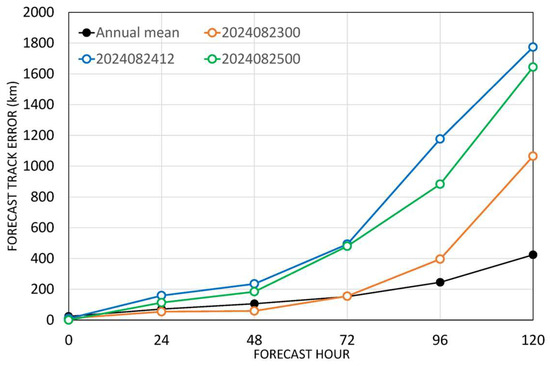
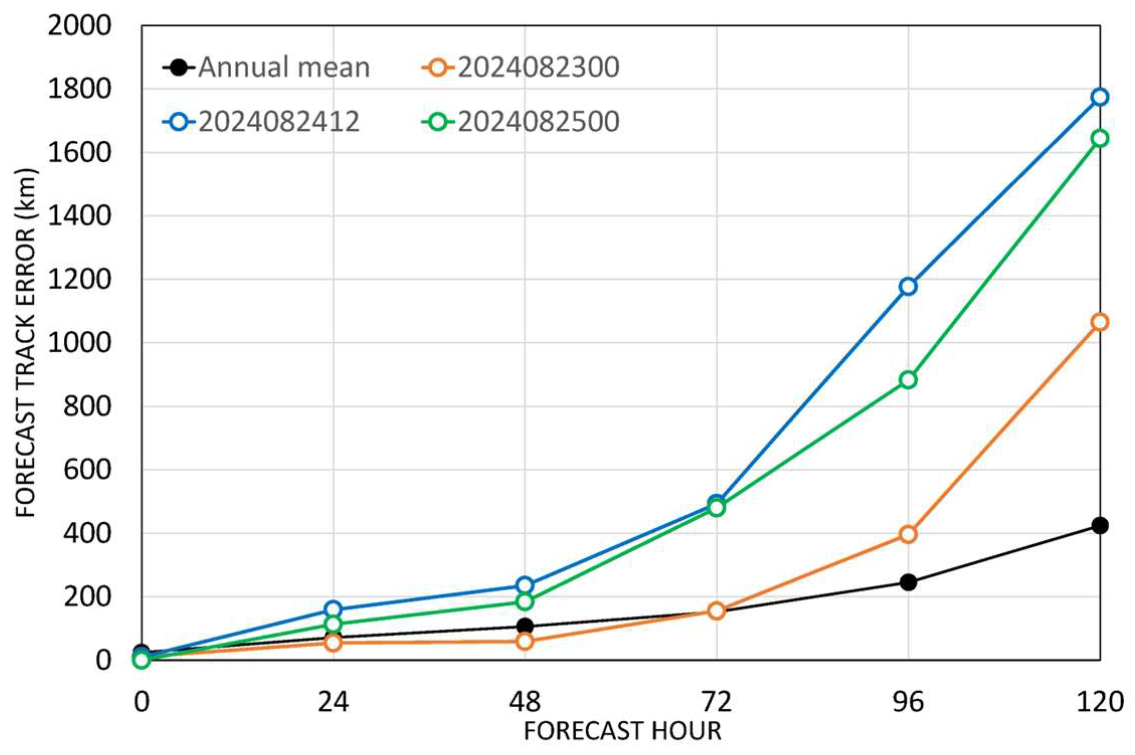
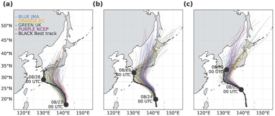
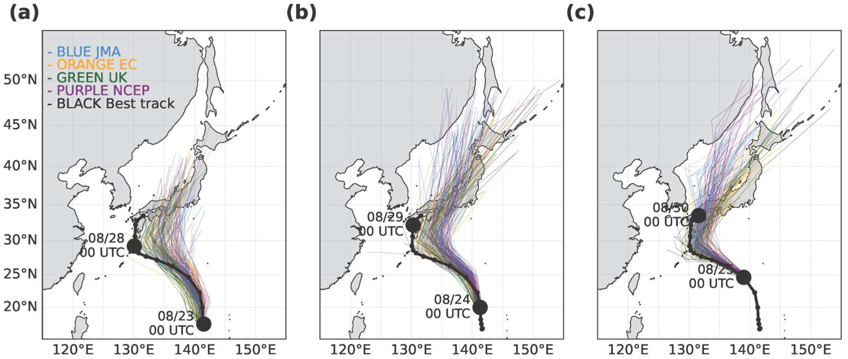
We examine ensemble track predictions for three initialization/target-time pairs associated with large 5-day track errors: at 00 UTC on 28 August (initial time: 00 UTC on 23 August), at 12 UTC on 29 August (initial time: at 12 UTC on 24 August), and at 00 UTC on 30 August (initial time: at 00 UTC on 25 August). For these cases, track errors tend to increase rapidly beyond 72 h (Figure 1). Almost all of the ensemble track predictions included in the grand ensemble failed to predict the extent of SHANSHAN’s westward movement in the intensification phase and exhibited a northeastward trend compared to RSMC-Tokyo best track (Figure 2).
Figure 1.
Time-series of forecast track errors (km) relative to the RSMC–Tokyo best track for Typhoon SHANSHAN (2024) as a function of forecast hour (FT). Annual mean errors indicate the mean errors in 2024.
Figure 2.
Tracks of SHANSHAN (black) for all 151 members as predicted by ECMWF (orange), JMA (blue), NCEP (purple), and UKMO (green). Panels show (a) target 28 Aug 00 UTC (initial: 00 UTC on 23 August), (b) target 29 Aug 12 UTC (initial: 12 UTC on 24 August), and (c) target 30 Aug 00 UTC (initial 00UTC on 25 August).
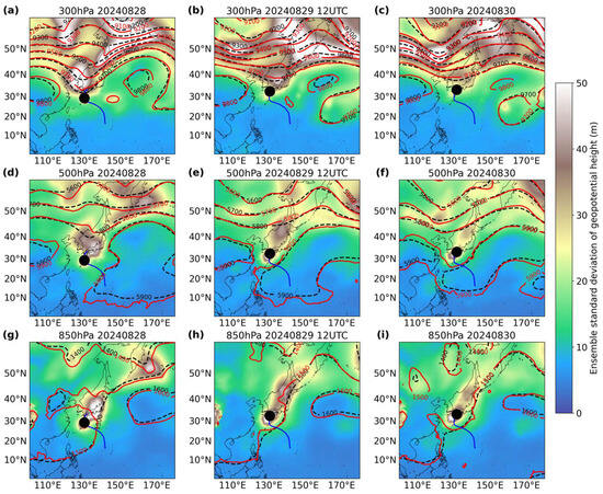
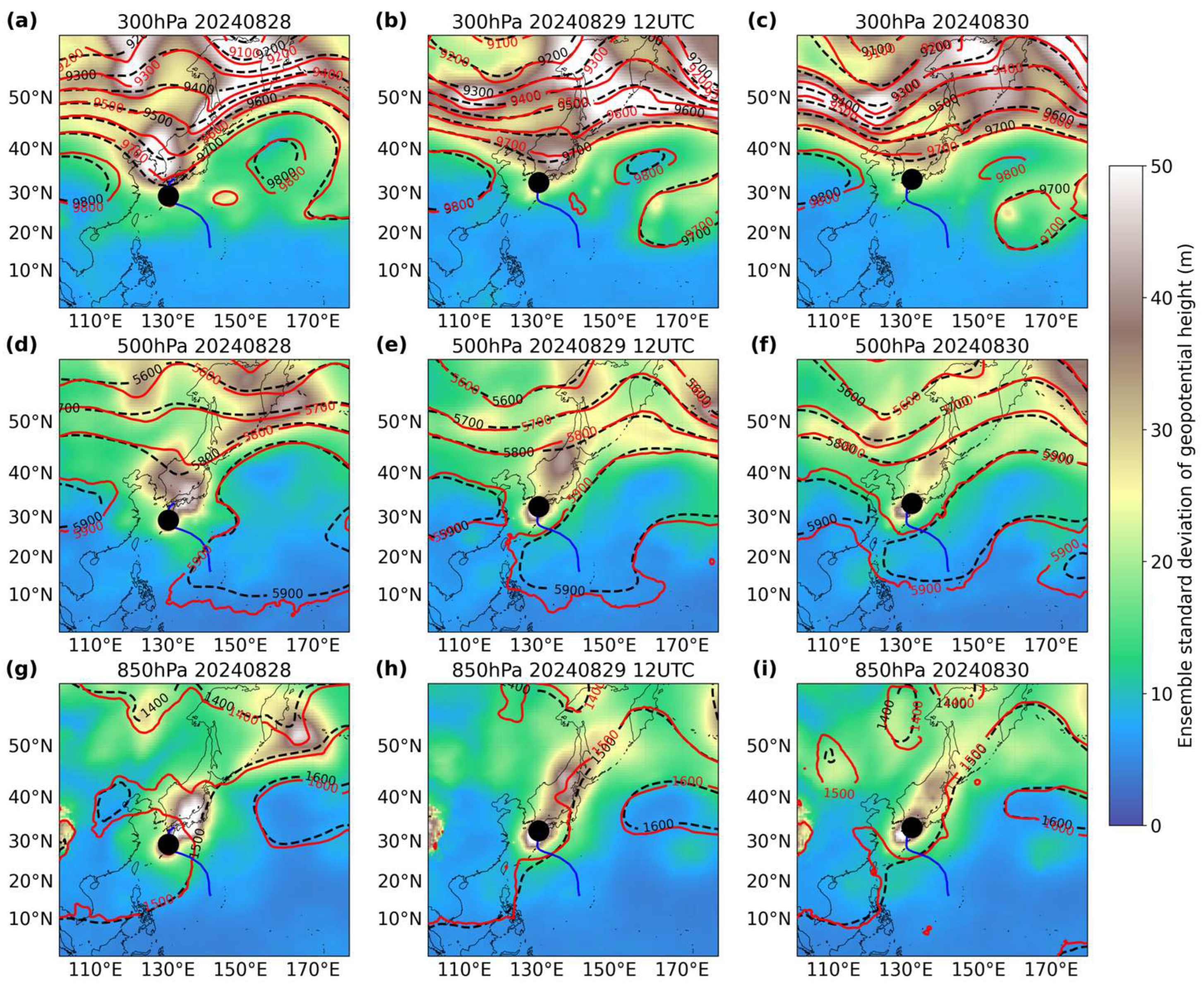
Figure 3 shows the horizontal distributions of standard deviations of geopotential height across the grand ensemble at the 300, 500, and 850 hPa pressure levels. The result also indicated that the grand ensemble mean fields at the three pressure levels are comparable to the ERA5 atmospheric reanalysis field. However, irrespective of the target time and pressure level, uncertainty is larger in the mid-latitudes than in the tropics. In addition, it is enhanced near the mid-latitude trough and around SHANSHAN, particularly at the 850 hPa pressure level. The result implies that errors in predicting the trough and the storm’s intensity-dependent lower-tropospheric structure both possibly contribute to uncertainty of track predictions.
Figure 3.
Horizontal distributions of geopotential height (red solid contours: ERA5; black dashed contours: ensemble mean) and ensemble spread (shading) at (a–c) 300, (d–f) 500, and (g–i) 850 hPa pressure levels for the three target times: (a,d,g) 00 UTC on 28 August, (b,e,h) 12 UTC on 29 August, and (c,f,i) 00 UTC on 30 August. The layout is organized by level (rows) and target time (columns).
To guide the subsequent EOF-based diagnosis, the synoptic features in Figure 3 are explored at each pressure level. At the 300 hPa pressure level, the ensemble spread is concentrated along the upper-tropospheric trough over the mid-latitudes around 130° E, indicating substantial uncertainty in the amplitude and longitudinal position of the mid-latitudinal jet–trough system including the location of jet streaks. At the 500 hPa height, the spread around the mid-latitudinal jet–trough system is relatively weak compared to that at the 300 hPa pressure level although the spread is still apparent around the Japanese archipelago. East of the apparent spread, the subtropical ridge represented by the geopotential height of 5900 m becomes apparent particularly at 12 UTC on 29 August and 00 UTC on 30 August. At the 850 hPa pressure level, the spread around the mid-latitudinal jet–trough system is not apparent, whereas the spread near SHANSHAN and another storm still remain particularly over the Japanese archipelago. The lower-tropospheric circulation over the continental monsoonal low over East Asia is found instead (Figure 3g–i). These level-dependent features provide physical context for the leading EOF modes in the following section and help explain why different modes dominate the westward-moving phase at 00 UTC on 28 August and the post-landfall eastward-moving phase at 12 UTC on 29 August and 00 UTC on 30 August. The case study and numerical experiment evidence likewise highlight the role of mid-latitude upper-level trough or cut-off low in governing TC track changes and forecast difficulty in the western North Pacific [15,16]. Similar links between mid-latitude trough representation and large TC track errors have been documented in other basins as well, for example, during Hurricane Joaquin (2015) using high-resolution Hurricane Weather Research and Forecasting (HWRF) ensembles [17].
4.2. Leading EOF Structures and Vertical Dependence
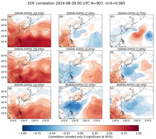
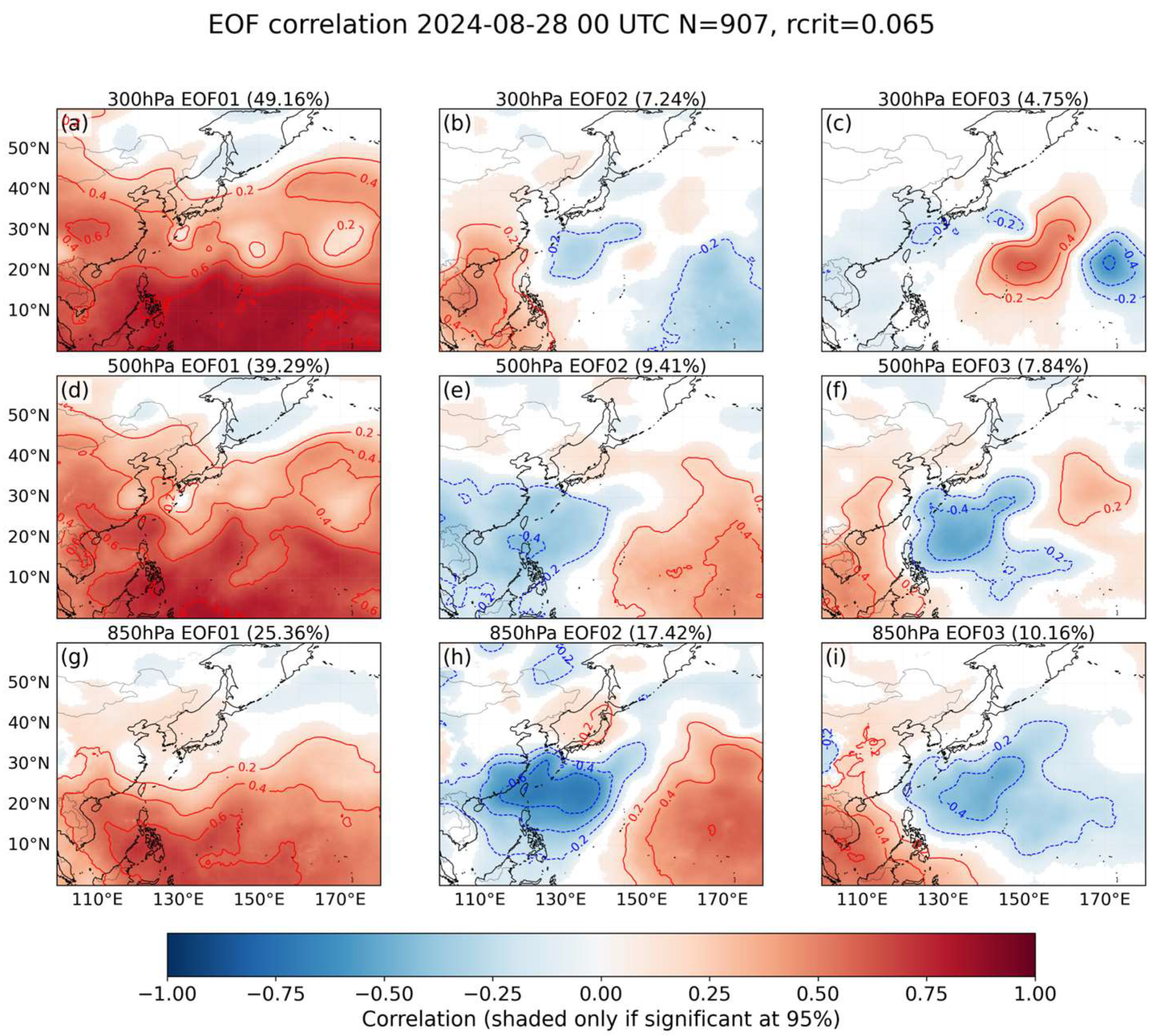
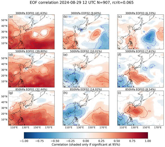
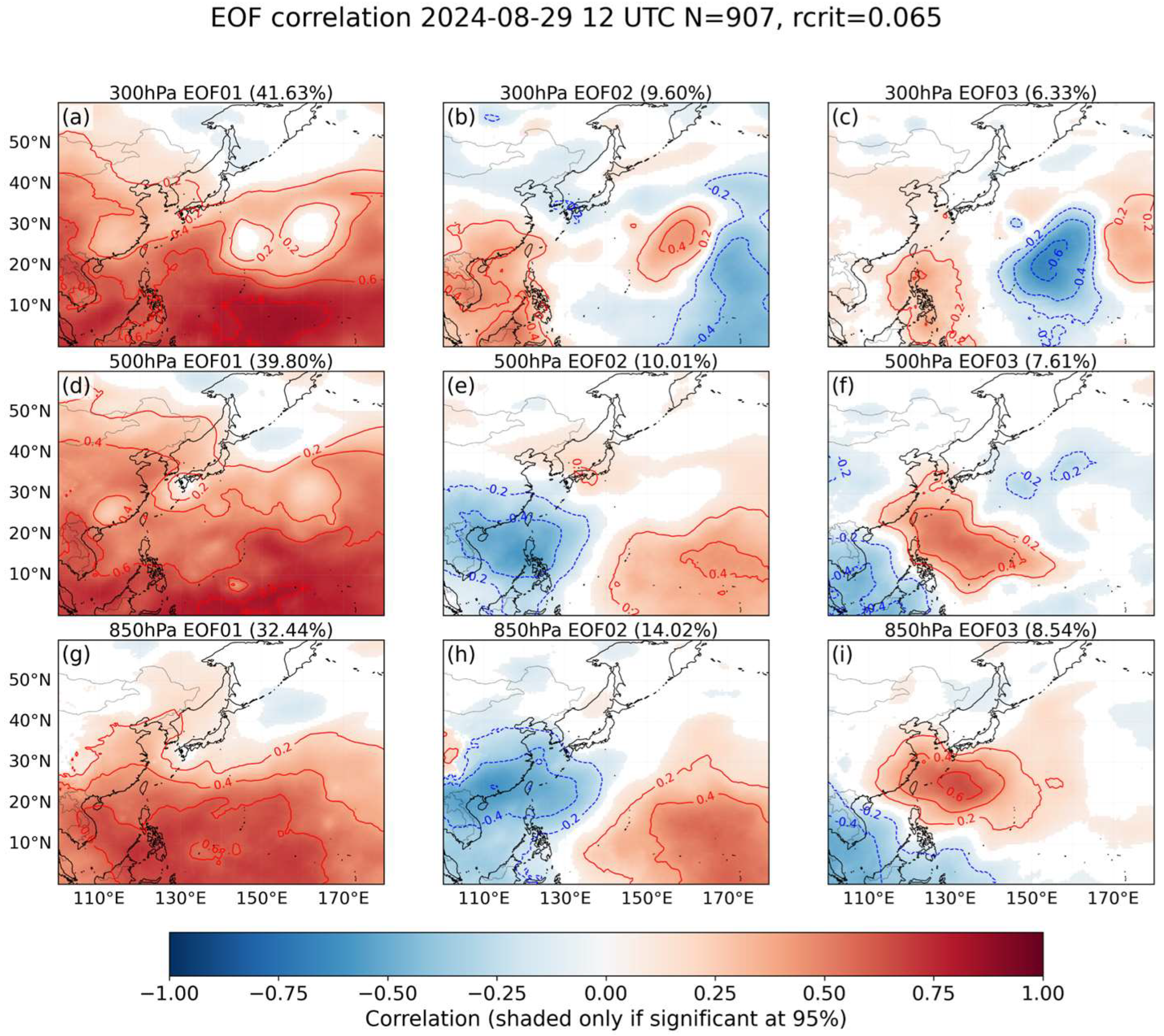
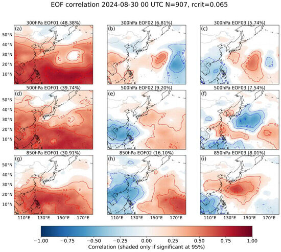
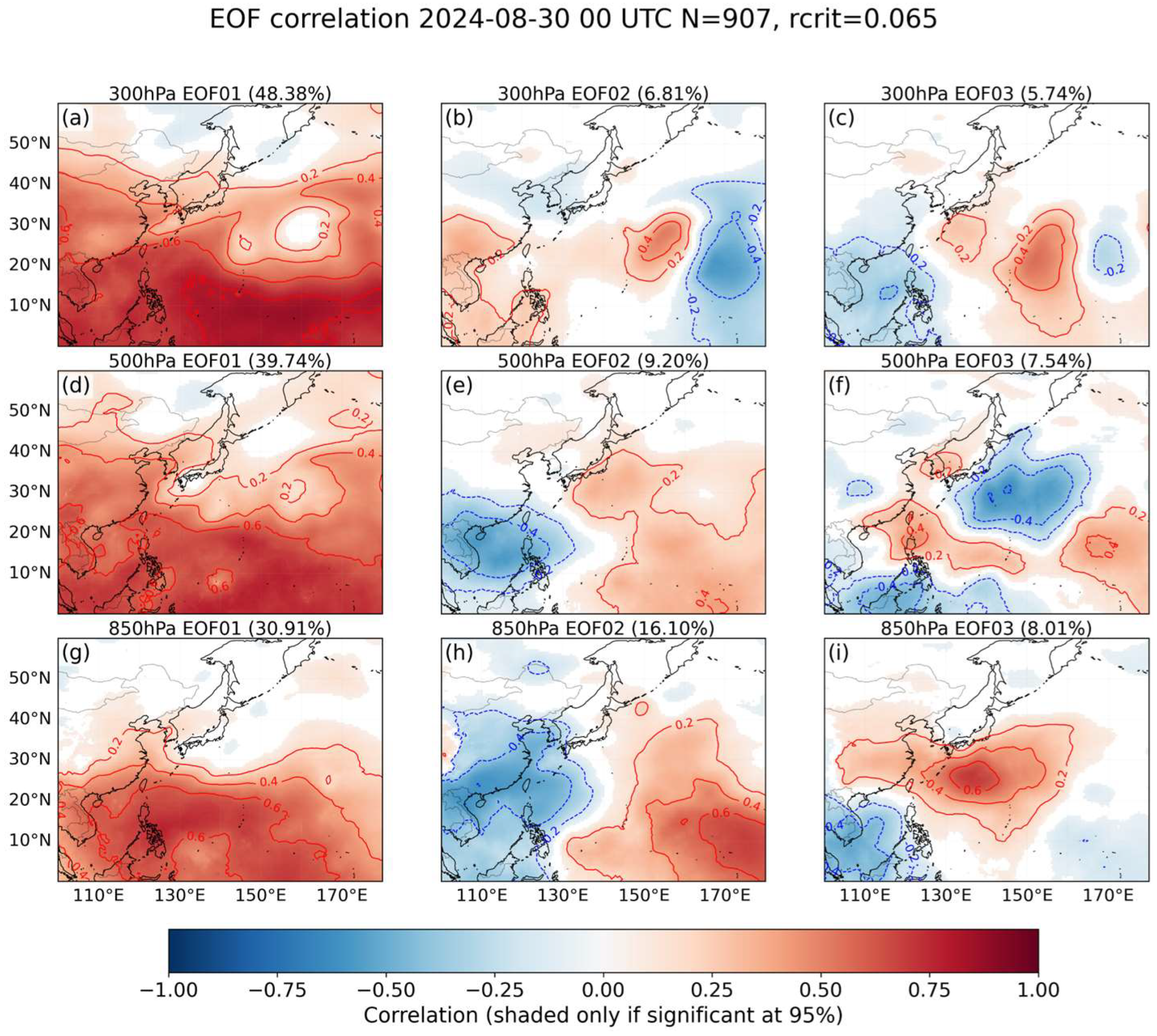
Figure 4, Figure 5 and Figure 6 show the horizontal distributions of EOF correlation at the significant level of 95% at the 300, 500, and 850 hPa pressure levels. At all three target times, EOF1 explains a substantially larger fraction of the variance than subsequent modes, especially in the upper troposphere (300 hPa pressure level). EOF1 exhibits a clear north–south asymmetric pattern, consistent with the contrast between tropical and mid-latitude variability. From the middle to lower troposphere, the explained variance fraction of EOF1 decreases and the relative contributions of EOF2/EOF3 increase, indicating that multiple modes are needed to understand lower-tropospheric uncertainty. Spatial patterns in EOF modes, higher than EOF3, exhibit smaller spatial structures than those in EOF1–3 modes.
Figure 4.
EOF1–EOF3 correlation with ERA5 at 300, 500, and 850 hPa pressure levels for 00 UTC on 28 August for all 907 members. Shading shows correlations significant at 95% (the value is higher than “rcrit”); non-significant areas are masked. Row order is a pressure level of 300, 500, and 850 hPa; column order is an EOF mode of EOF1, EOF2, EOF3. Panel labels (a–i) follow row-major order.
Figure 5.
Same as Figure 4 but for 12 UTC on 29 August.
Figure 6.
Same as Figure 4 but for 00 UTC on 30 August.
Furthermore, EOF1–3 show nearly identical spatial patterns across the different initial times, whereas the spatial patterns of EOF4–10 vary depending on the initial time (Figures S1–S3). This indicates that the differences observed in the grand ensemble can be primarily explained by three spatial EOF patterns, regardless of the initial time or numerical prediction system used. Meanwhile, the existence of higher-order EOF modes indicates the presence of a group sharing a common variability pattern in the grand ensemble, potentially supporting the existence of differences caused by initial conditions and numerical prediction system. Inter-center contrasts in ensemble sensitivity structure have been documented for recent western North Pacific cases, with ensemble prediction system (EPS)-dependent behaviors linked to synoptic feature representation and model error [18].
4.3. PC Space Representation and Track Error Labels
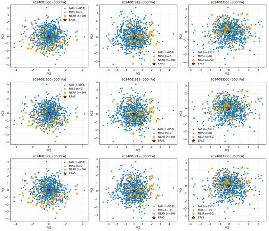
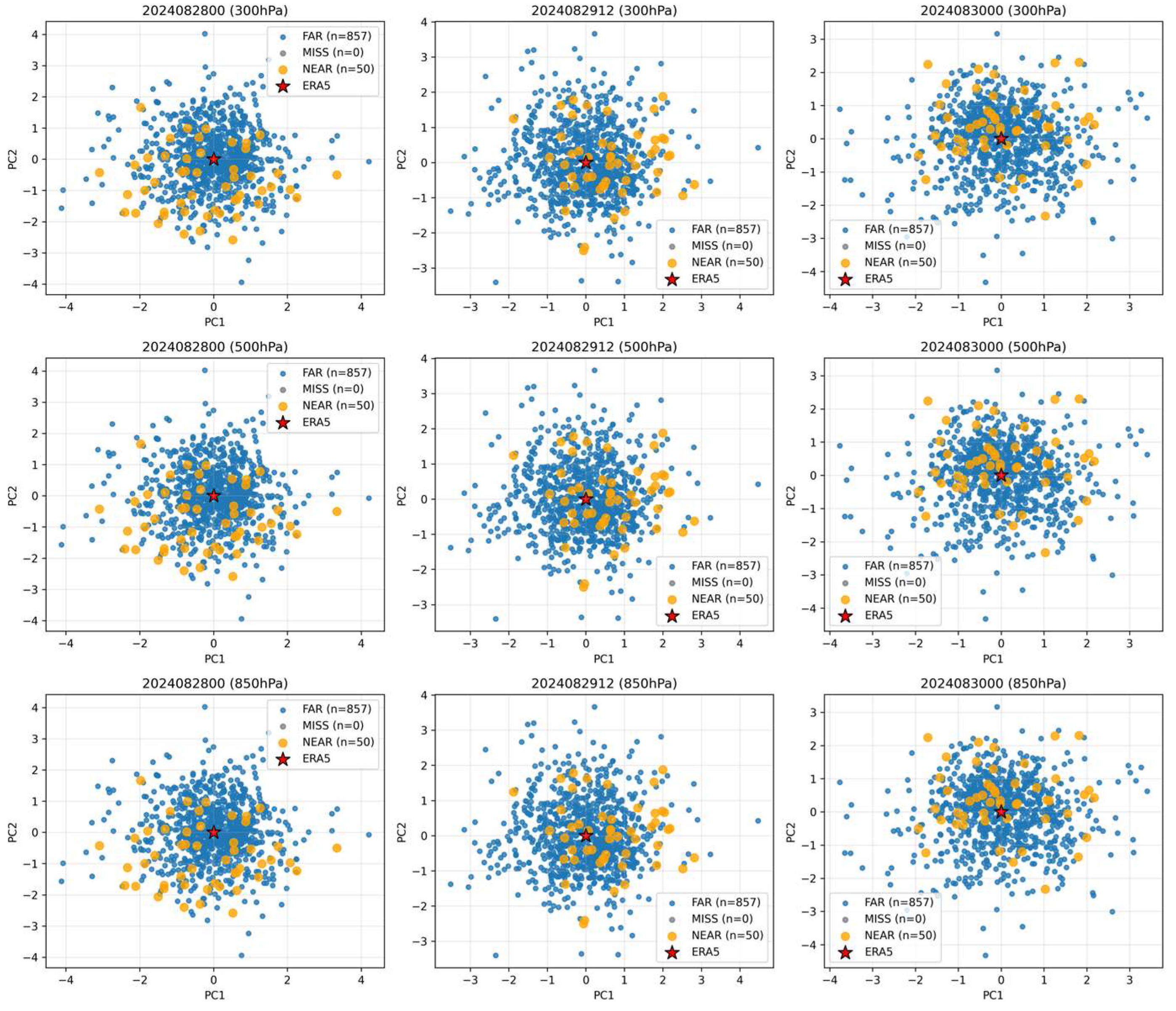
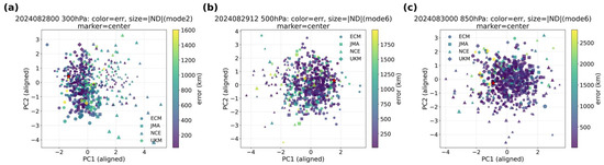
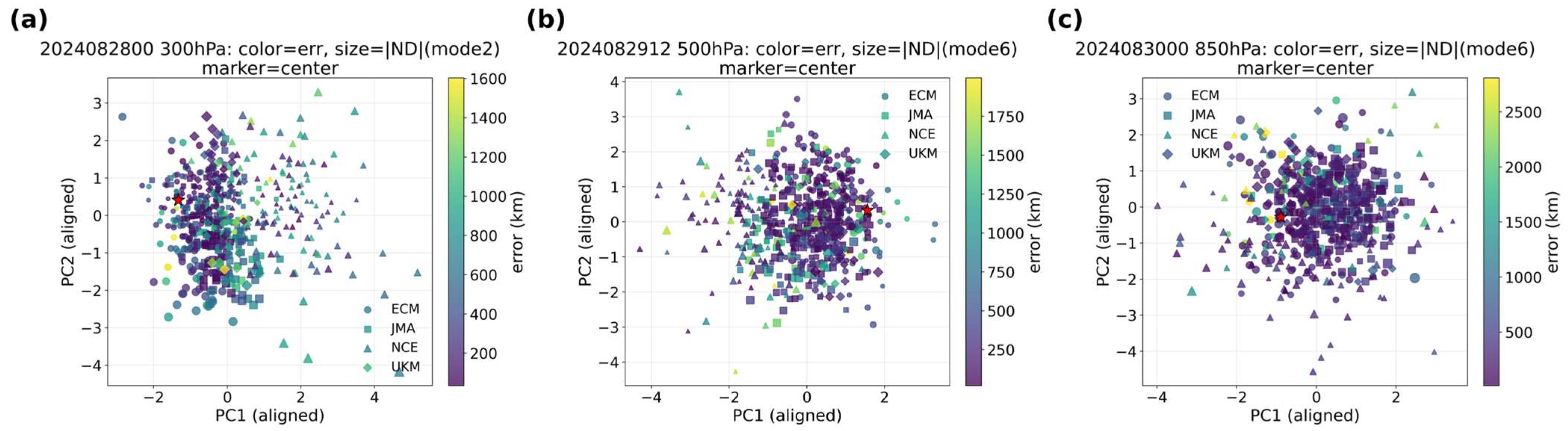
The EOF correlation maps in Figure 4, Figure 5 and Figure 6 indicate that the leading EOF1-EOF3 modes are relatively stable across target times, whereas higher-order modes (EOF4–EOF10) exhibit stronger time dependence (Figures S1–S3). To connect these mode characteristics to track-forecast outcomes, we next show a scatter diagram of the grand ensemble members and ERA5 in a low-dimensional PC1–PC2 space at each target time. The distribution in the PC1–PC2 plane also shows the track error labels (“NEAR”, “FAR”, “MISS”) defined in Section 3.1.
Figure 7 shows that grand ensemble members are broadly scattered around the ERA5 location in the low-order PC1–PC2 space at each target time, indicating substantial diversity in the dominant synoptic patterns even within a low-dimensional representation. The spread suggests that multiple realizations of the large-scale environment coexist in the ensemble, reflecting uncertainty that is relevant to SHANSHAN’s location. Proximity to the ERA5 point in the PC1–PC2 space does not uniquely correspond to small track error. It should also be emphasized that proximity to ERA5 in the aligned PC space does not guarantee small track errors, as already shown in Figure 7. This indicates that the relationship between synoptic structure similarity and track prediction skill is not trivial, and that the effectiveness of the proposed conditioning reflects the selective extraction of dynamically relevant structures rather than a simple confirmation of ERA5 quality. In fact, members located near ERA5 in the PC1–PC2 space can still be labeled as “FAR” or “MISS”, while some “NEAR” members may occur away from the immediate ERA5 neighborhood. This indicates that track error outcomes are not determined solely by agreement in the first two representative PCs. The result is also seen in PC1–PC3 and PC2–PC3 spaces. Therefore, matching only the dominant, quasi-stationary variability patterns represented by the leading EOF modes to ERA5 is informative but not sufficient to guarantee improved track prediction. Residual differences in higher-order modes can still project onto the track error, which motivates the subsequent analysis that explicitly considers higher-order modes and their rotational alignment before performing ERA5-consistent member selection.
Figure 7.
PC space (PC1–PC2) distribution of grand ensemble members and ERA5 (red star) at each target time at three pressure levels; point color denotes PC3. Members are labeled “NEAR” (orange circles), “FAR” (blue circles), “MISS” (gray circles) based on track position error at the corresponding valid time (see Section 3.1). Panels: (left column) 00 UTC on 28 August, (middle column) 12 UTC on 29 August, (right column) 00 UTC on 30 August, (top row) 300 hPa level, (middle row) 500 hPa level, (bottom row) 850 hPa level.
4.4. Inter-Center Differences in PC Amplitudes
We define the three member groups used for conditional evaluation of track error statistics. “All” denotes the full candidate population used for conditioning at each target time (restricted to members with FT = 48, 72, 96, and 120 h as described in Section 3.2). “Good” denotes a subset of members selected as most consistent with ERA5 in the PC space according to a specified similarity criterion (Section 3.2). “Intersection” denotes the overlap of “Good” subsets obtained from two different similarity criteria (i.e., members selected by both criteria) and is used to identify members that are robustly ERA5-consistent across definitions. Note again that these selection-based groups (“All”, “Good”, “Intersection”) are conceptually distinct from the outcome-based track error labels (“NEAR”, “FAR”, “MISS”; Section 3.1) used for visualization in Figure 7.
In multi-time PC comparisons, the choice of a reference EOF basis is not unique. In this study, the earliest target time (00 UTC on 28 August) is adopted as the reference. This is because the leading EOF modes at this time exhibit the smallest principal angles relative to the other target times. In addition, the synoptic-scale structure is most stable in the early phase. Furthermore, using the earliest phase as the baseline provides a physically meaningful anchor for describing the subsequent evolution of the synoptic-scale environment.
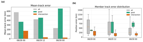
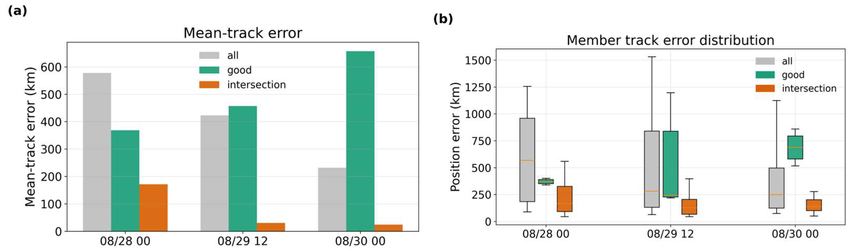
Figure 8 shows how conditioning the grand ensemble on reanalysis consistency affects SHANSHAN’s track errors at the three target times. In Figure 8a, the mean track error is compared among “All”, “Good”, and “Intersection”. In Figure 8b, the distributions of member track errors are shown for the same three groups. Overall, the “Good” subset exhibits reduced track errors relative to “All”, and the “Intersection” subset tends to provide the smallest errors, indicating that the improvement is robust across selection definitions. The distributional view further highlights that conditioning primarily suppresses the large-error tail or “forecast-bust outliers” rather than merely shifting the mean.
Figure 8.
(a) Mean track error (km) for “All” and “Good”(Mahalanobis) and their “Intersection” (Mahalanobis ∩ z-Euclid) at each target time; (b) distributions of member track errors for the same groups, illustrating suppression of the large-error tail by ERA5-consistent.
Therefore, while the low-order PC representation provides a useful entry point, the results in Figure 8 motivate a deeper analysis of which aspects of the synoptic variability control the phase-dependent forecast errors and the track-skill improvement under conditioning. In particular, agreement in the first few EOF modes alone is not sufficient to guarantee small track errors (as suggested by Figure 7), which points to the potential importance of higher-order, time-dependent modes.
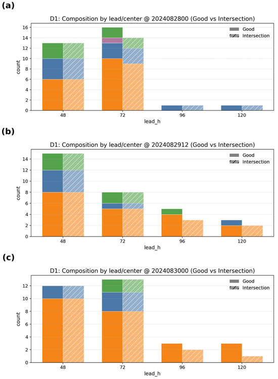
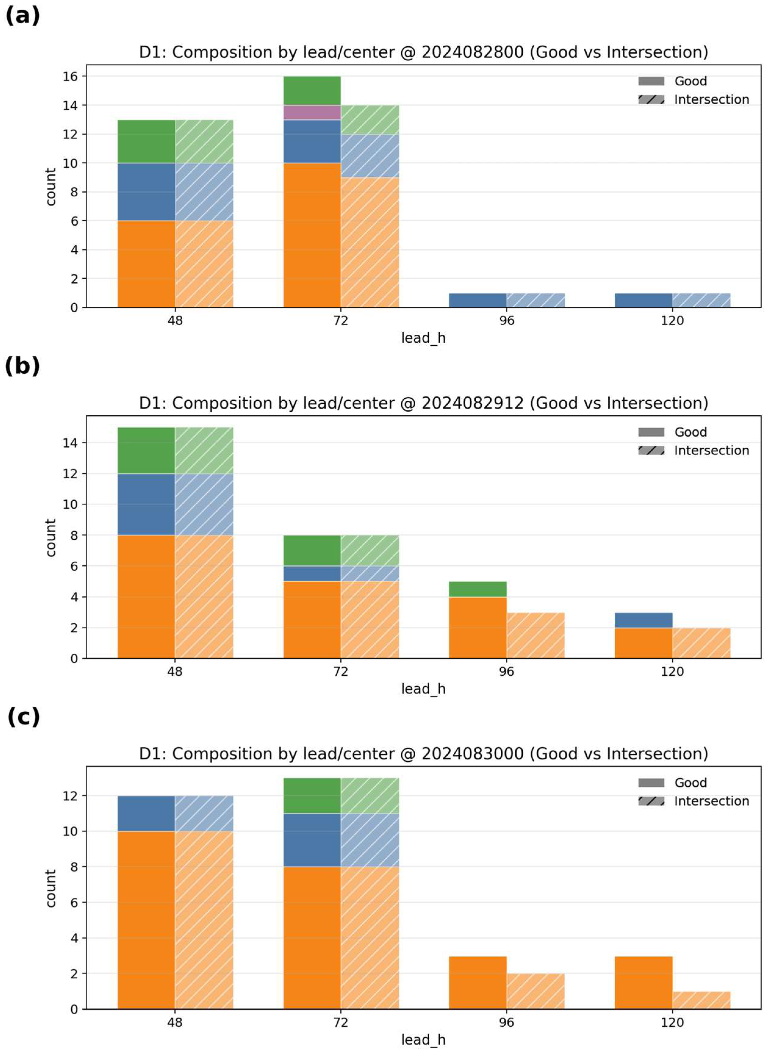
To understand which forecast centers and lead times contribute to the improvement shown in Figure 8, it is necessary to examine the composition of the selected “Good” members. This decomposition clarifies where the ERA5-consistent members originate and provides insight into why the conditional selection is effective. Figure 9 shows the composition of the selected “Good” members in terms of forecast center (ECMWF, JMA, NCEP, UKMO) and forecast lead time (FT = 48, 72, 96, and 120 h). Across all three target times, “Good” members originate predominantly from ECMWF and JMA, whereas NCEP contributes only a small fraction. This is broadly consistent with the difference in normalized amplitudes noted in the upper-level modes (Figure 4, Figure 5 and Figure 6). The result suggests that differences in the representation of upper-tropospheric structures affect the degree of similarity to ERA5 in PC space.
Figure 9.
Composition of “Good” members by forecast center (ECMWF (orange)/JMA (blue)/NCEP (purple)/UKMO (green)) and lead time (48/72/96/120 h) at (a) 00 UTC on 28 August, (b) 12 UTC on 29 August, and (c) 00 UTC on 30 August.
4.5. PC Space Structure and Distance-Based Selection
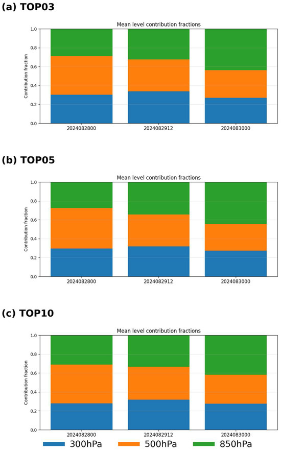
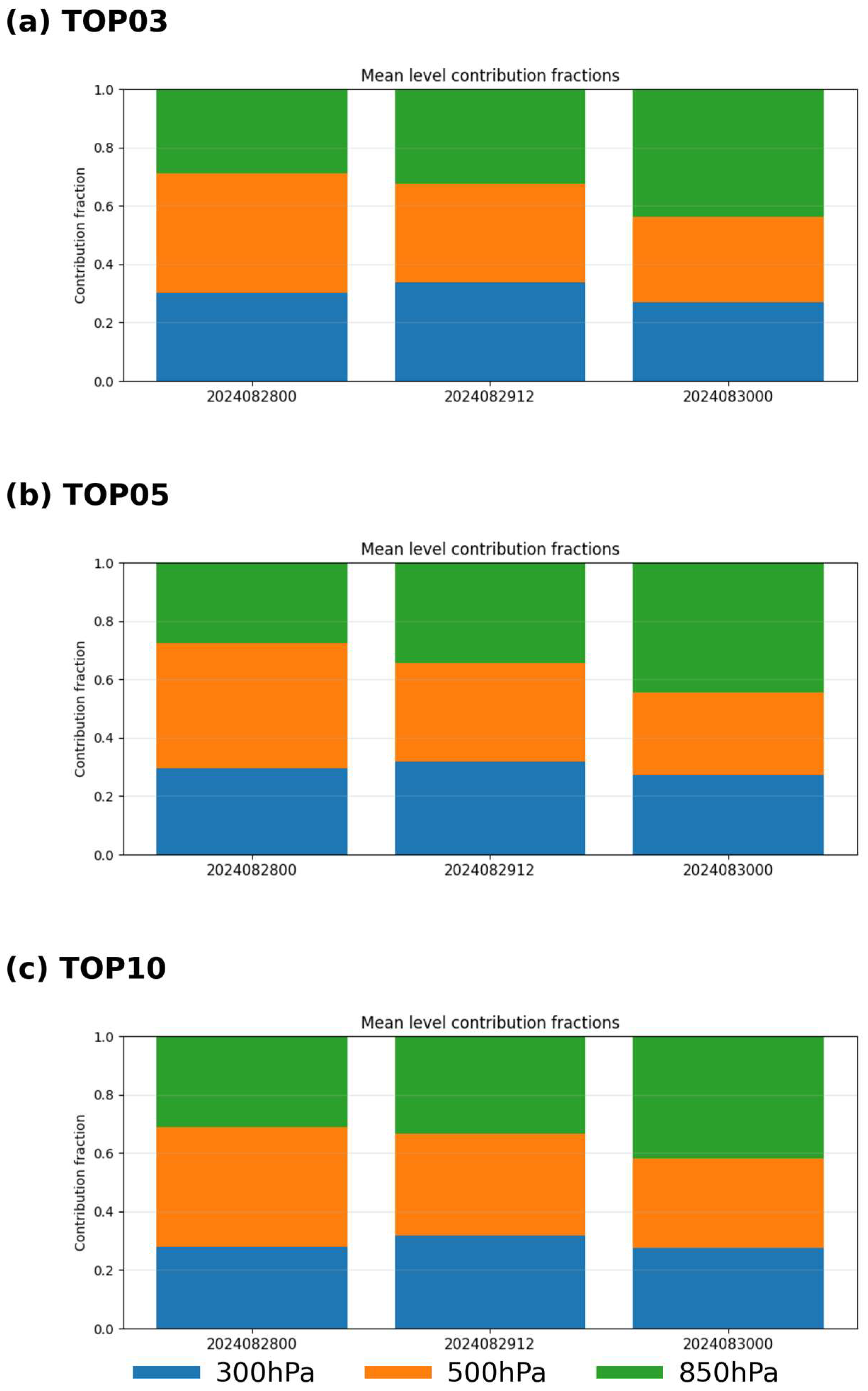
We use the term ΔRecon in Equation (11) to denote the reconstructed-field difference in the reference EOF space between the “Good” and “All” subsets using the reference-time modes. Positive or negative values in ΔRecon indicate the direction in which the “Good” subset modifies the synoptic structure relative to “All”, allowing interpretation of whether specific synoptic features (e.g., trough amplitude or ridge position) are strengthened or weakened. EOFs are sign-aligned and defined on the reference-time basis. This mode-conditioned reconstruction provides a complementary view to piecewise potential vorticity (PV) inversion diagnostics that attribute steering flow errors to specific synoptic systems [19]. Figure 10 shows the relative contributions of the 300, 500, and 850 hPa pressure levels to the track error improvement obtained through the “Good” selection, together with their sensitivity to the selection threshold. Panels (a–c) correspond to the top 3%, 5%, and 10% subsets, respectively. For all thresholds and target times, the level-wise contributions are distributed from the lower to upper troposphere, indicating that the improvement is not dominated by a single level but is instead supported by multi-level information. This qualitative vertical structure is robust across different thresholds. The relative magnitudes, however, differ by TC phase and are moderately affected by the threshold choice.
Figure 10.
Sensitivity of level contribution diagnostics (300, 500, and 850 hPa) to the selection threshold. Panels (a–c) show results for the top 3%, 5%, and 10% subsets, respectively. Bars indicate the mean fractional contribution of each level to the total error reduction from “All” to “Good” at each target time.
At 00 UTC on 28 August, the 850 hPa contribution is comparatively larger, consistent with the enhanced lower-tropospheric spread around SHANSHAN noted in Figure 3 and with the importance of EOF2 and EOF4 variability during the westward-moving phase. In contrast, at 12 UTC on 29 August and 00 UTC on 30 August, the 300 and 500 hPa pressure levels contribute more strongly, reflecting the upper- and mid-tropospheric uncertainty associated with the eastward progression after recurvature and landfall. Increasing the threshold (e.g., top 10%) tends to slightly enhance the contrast between levels, whereas smaller subsets (top 3%) yield smoother distributions, but the overall phase-dependent structure remains consistent. The 5% threshold provides a representative balance between stability and contrast.
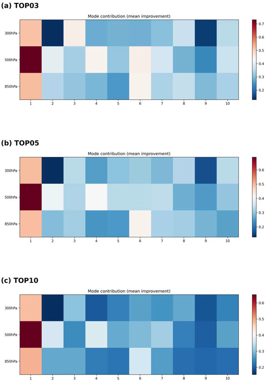
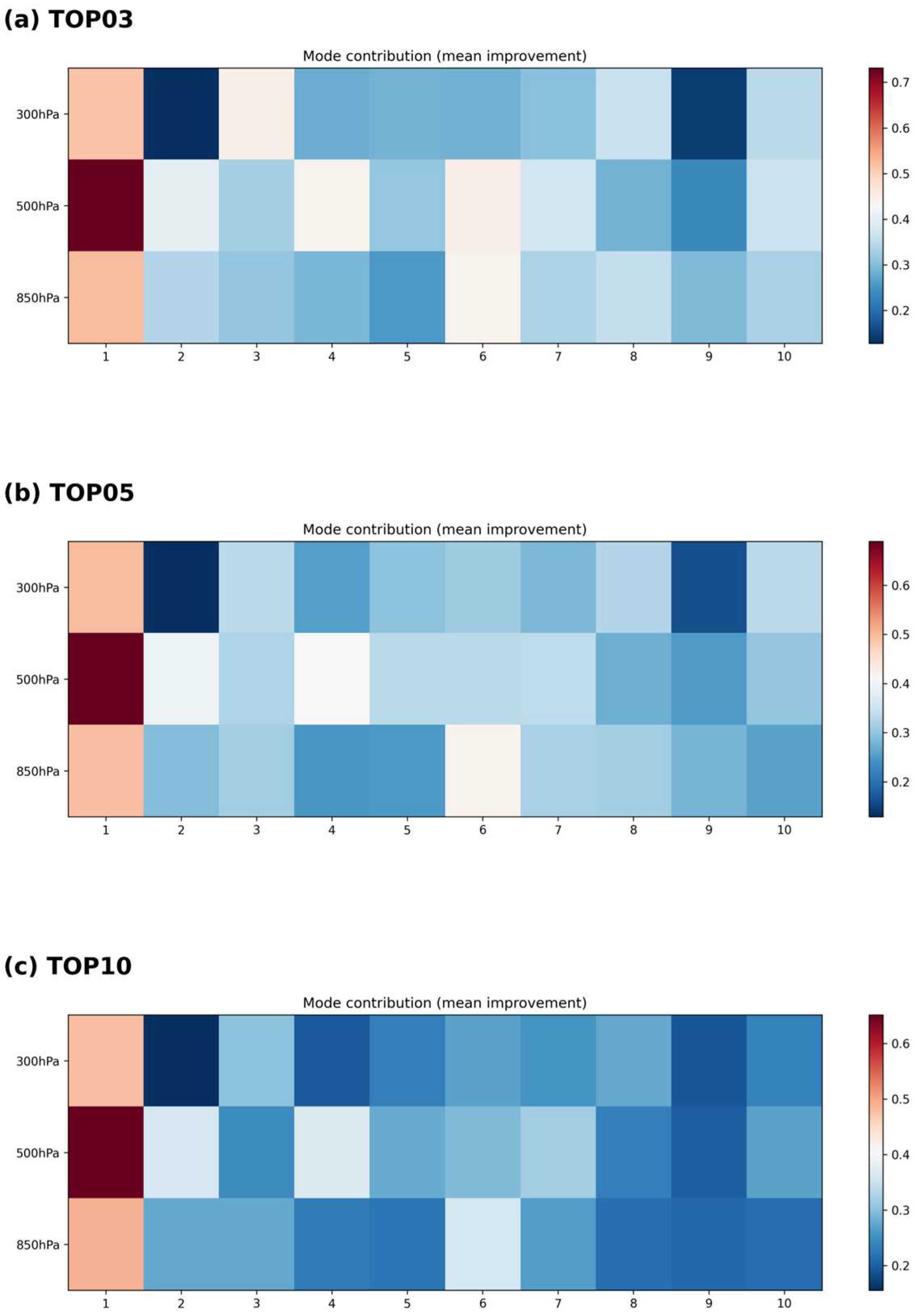
Figure 11 shows the relative contributions of individual EOF modes (1–10) to the improvement obtained by the “Good” selection at each target time, together with their sensitivity to the selection threshold (top 3%, 5%, and 10% in panels (a–c), respectively). Each cell reports a z-score-normalized mode-wise contribution in Equation (13) to the error reduction from “All” to “Good”; positive (blue) indicates improvement, whereas negative (red) indicates degradation. The color scale is symmetric and saturated at the 95th percentile of the absolute value of the contribution. The heat map structure reveals pronounced phase dependence in the effective modes, which is qualitatively consistent across thresholds but shows stronger variability than the level-based diagnostics. At 00 UTC on 28 August, EOF2 and EOF4 emerge as major contributors after EOF1, highlighting their role in representing lower-tropospheric and mid-latitude trough variability during the westward-moving phase of SHANSHAN. At the later target times, the dominant contributors shift to EOF6 and EOF7, consistent with the enhanced importance of upper- and mid-tropospheric structures during the post-landfall eastward-progression phase. EOF1 contributes substantially at all times across all thresholds, reflecting its role in capturing the large-scale background structure described in Section 4.2. In contrast to the level-based contributions, the magnitude and spatial patterns of higher-order modes (particularly beyond EOF7) exhibit stronger sensitivity to the threshold choice, with larger subsets (top 10%) showing enhanced contrasts and increased variability, and smaller subsets (top 3%) showing reduced contrast. These results indicate that while the dominant mode structures are robust, the detailed distribution of contributions across higher-order modes is sensitive to the selection criterion. This behavior supports the interpretation that the improvement gained by conditioning on ERA5-consistent members arises from coherent multi-level synoptic structure, with additional sensitivity in the modal representation of that structure.
Figure 11.
Sensitivity of mode contribution patterns to the selection threshold. Panels (a–c) correspond to the top 3%, 5%, and 10% subsets. The heat maps show the z-score-normalized contribution of each EOF mode (1–10) to the error reduction from “All” to “Good” at each target time. Blue indicates improvement and red indicates degradation, with the color scale symmetric and saturated at the 95th percentile of the absolute contribution.
It should be noted that the mode-wise contributions shown in Figure 11 represent statistical measures in the aligned PC space and do not directly convey the physical structures associated with each mode. In addition, the specific EOF mode numbers identified in this study (e.g., EOF2, EOF4, EOF6, EOF7) are not universal and depend on the dataset, domain, and target time. In contrast, the physical structures represented by these modes—such as lower-tropospheric circulation near the storm and upper- to mid-tropospheric wave–trough systems—are more general and provide a physically interpretable basis for understanding phase-dependent forecast errors. Thus, the primary implication of this study lies in the identification of phase-dependent synoptic structures rather than in the specific mode indices themselves.
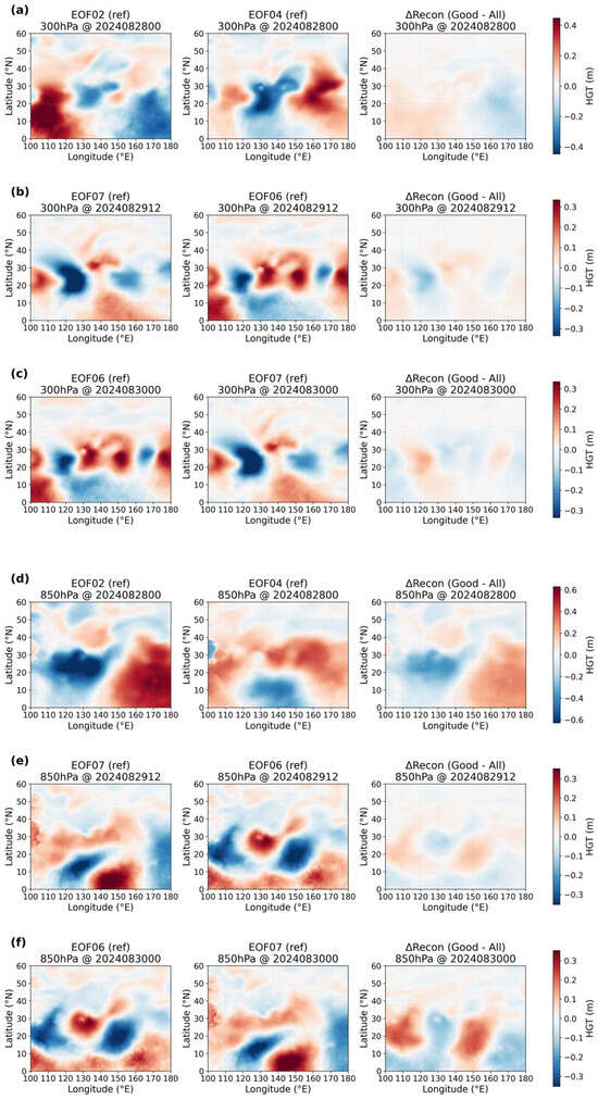
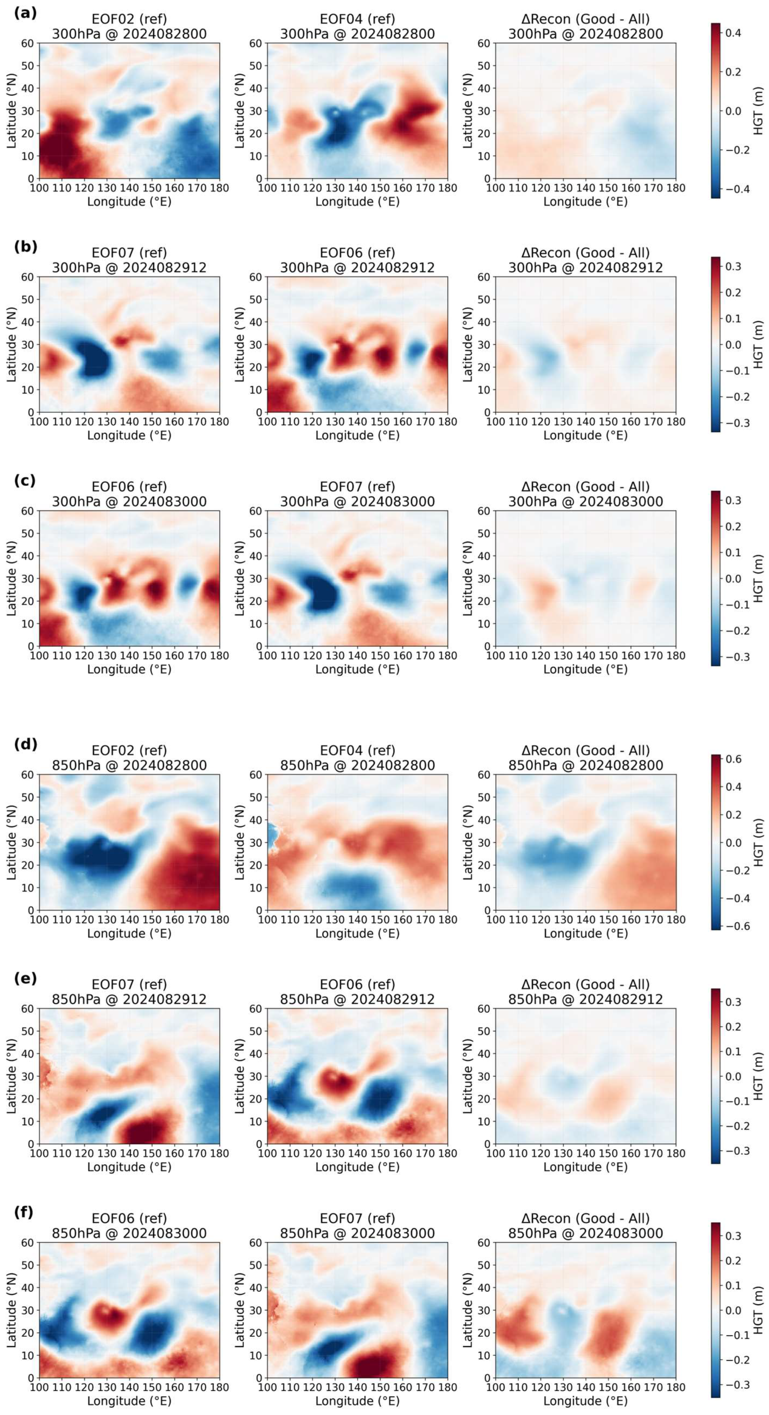
Figure 12 compares representative EOF patterns with the reconstructed-field differences between the “Good” and “All” subsets (ΔRecon = “Good” − “All” calculated in Equation (11)) for the two phases. For 00 UTC on 28 August in a westward-moving phase, EOF2 and EOF4 emerge as the primary contributors after EOF1 and correspond to lower-tropospheric structure near SHANSHAN and the neighboring mid-latitude trough. Their spatial polarity matches the sign of the ΔRecon fields, indicating that members selected as ERA5-consistent reduce the displacement/amplitude error of these features. For 12 UTC on 29 August in a post-landfall eastward-progression phase, the dominant contributors shift to EOF6 and EOF7, highlighting upper-/mid-tropospheric wave structures; the ΔRecon maps show that the “Good” subset mitigates the phase and amplitude biases of the trough–ridge system aloft. Therefore, Figure 12 provide a physical bridge from the statistical diagnostics in Figure 10 and Figure 11 to the large-scale circulation elements that govern the phase-dependent track errors. These physically interpreted structures are consistent with the mode-wise contributions identified in Figure 11, providing a coherent link between the statistical diagnostics in PC space and the underlying synoptic dynamics.
Figure 12.
Representative EOF patterns (left in each pair) and reconstructed-field differences (ΔRecon = “Good” − “All”, right) for (a,d) 00 UTC on 28 August (EOF2, EOF4), (b,e) 12 UTC on 29 August (EOF7, EOF6), and (c,f) 00 UTC on 30 August (EOF6, EOF7) at the 300 hPa (a–c) and 850 hPa (d–f) pressure levels. Polarity match indicates which synoptic features (lower-tropospheric structure near SHANSHAN; mid-latitude trough–ridge aloft) are corrected by ERA5-consistent selection.
4.6. Similarity Versus Track Error and the Role of Mode Number
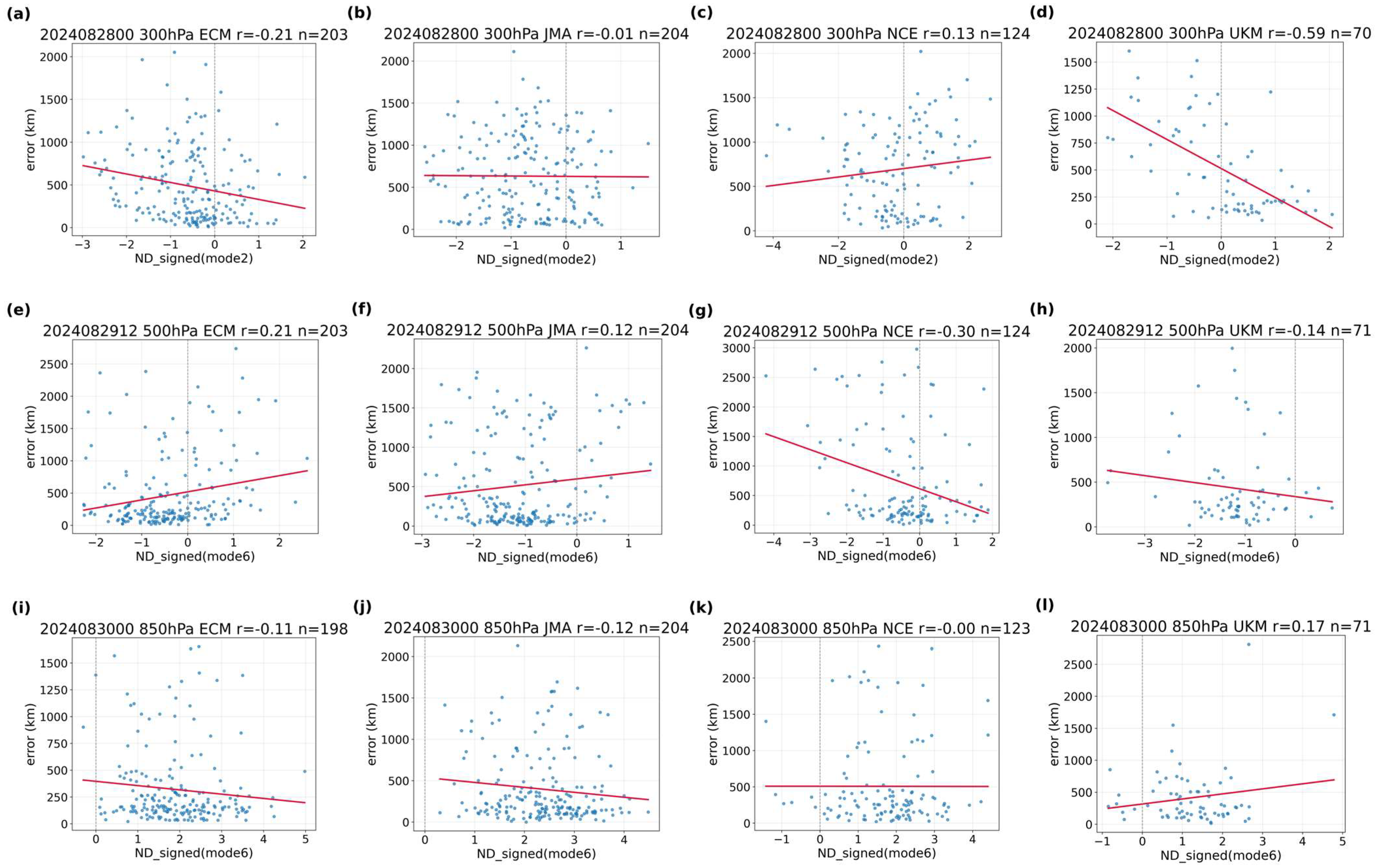
Building on the physical interpretation in Figure 12, we now quantify how mode-wise agreement with ERA5 in the aligned PC space translates into track error reduction. We first identify, for each target time, the “time × level × mode” combination that exhibits the strongest error association under balanced sampling across centers and then summarize the corresponding regressions. Figure 13 quantifies how signed normalized deviations from ERA5 in the aligned PC space relate to the track position error. For each target time, we display the “time × level × mode” combination that yields the largest absolute correlation under balanced sampling across centers. The three representative panels show that: (a) 00 UTC on 28 August: 850 hPa × EOF2 exhibits a negative association (larger agreement with ERA5 implies smaller error), consistent with the importance of the lower-tropospheric structure during the westward-moving phase; (b) 12 UTC on 29 August: 300 hPa × EOF7 shows the strongest association, indicating the key role of upper-tropospheric variability after landfall; (c) 00 UTC on 30 August: 500 hPa × EOF7 dominates, confirming the persistence of mid- and upper-level control during the later phase. The regression slopes and correlations are modest in magnitude—consistent with the multi-factor control of TC motion—but statistically coherent across phases and aligned with the mode-wise contributions in Figure 11 and the synoptic interpretation in Figure 12. It should be noted that all regressions use balanced subsamples across centers; repeated draws confirm that both median slopes and the correlation “r” are robust to mitigate unequal center sample sizes.
Figure 13.
Relationship between track position error (km) and signed normalized deviation from ERA5 (red star) in the aligned PC space (ND_signed) for the “time × level × mode” combination with the largest absolute correlation at each time: (a) 00 UTC on 28 August—850 hPa × EOF2; (b) 12 UTC on 29 August—300 hPa × EOF7; (c) 00 UTC on 30 August—500 hPa × EOF7.
At 00 UTC on 28 August, the EOF2/EOF4 polarity indicates that a west-shifted and deeper lower-tropospheric trough to the northwest of SHANSHAN, together with a weaker mid-tropospheric subtropical ridge to the east, corresponds to smaller track errors. In addition, ΔRecon shows that the “Good” subset suppresses the east-biased steering seen in “All”. In contrast, at 12 UTC on 29 August and 00 UTC on 30 August, the EOF6/EOF7 polarity highlights upper-/mid-tropospheric wave-packet phase; ERA5-consistent members reduce the downstream ridge over the Japanese archipelago and enhance the upstream trough, mitigating premature northeastward acceleration. These tendencies are consistent with the regression signs in Figure 13. The observed linkage between PC space deviations and track position errors is consistent with diagnostic frameworks showing that TC motion errors are primarily governed by environmental steering flow errors [20]. Idealized dynamics show that the TC–trough interaction depends on the relative distance/phase and amplitude/wavelength of the upper-level wave, consistent with the mid- and upper-level dominance seen after recurvature [21]. Therefore, the results close the loop from selection, contributions, synoptic interpretation, and error linkage, and thus a separate section is not presented here.
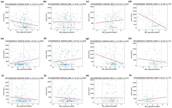
To complement Figure 13 and verify the robustness of the regression-based linkage between aligned PC deviations and the track position error, Figure 14 provides an additional set of scatter plot diagnostics. Specifically, it (i) repeats the regression with the same “time × level × mode” settings under alternative sampling/normalization choices, (ii) contrasts ordinary-least-squares lines with center-stratified fits to indicate inter-center spread, and (iii) annotates slope, Pearson correlation (r), and uncertainty bands to highlight where the signed deviation from ERA5 most coherently projects onto the error. Together with Figure 10, Figure 11, Figure 12 and Figure 13, this figure consolidates the phase-dependent control by lower-tropospheric modes at 00 UTC on 28 August and by mid-/upper-tropospheric modes at 12 UTC on 29 August and 00 UTC on 30 August, providing an internally consistent view from mode contributions to regression evidence.
Figure 14.
Scatter plots with fitted lines are shown for the same “time × level × mode” settings as in Figure 13, together with slope (β), Pearson correlation (r), and uncertainty bands. Where relevant, center-stratified fits are overlain to indicate inter-center spread. These panels corroborate the phase-dependent control highlighted earlier—larger agreement with ERA5 at the 850 hPa pressure level at (a–d) 00 UTC on 28 August and at the 300/500 hPa pressure levels on at (e–h) 12 UTC on 29 August and (i–l) 00 UTC on 30 August for (a,e,i) ECMWF, (b,f,j) JMA, (c,g,k) NCEP and (d,h,l) is associated with smaller track errors—serving as a robustness check for the regression-based interpretation.
5. Discussion
This single-case diagnosis provides a phase-aware link between ensemble spread in the synoptic environment and large track-forecast errors during SHANSHAN (2024). Three aspects are worth discussing.
- (i)
- Why phase-aware conditioning works
Figure 10, Figure 11 and Figure 12 demonstrate that the effective degrees of freedom of synoptic uncertainty change with the phase: during the westward-moving phase (00 UTC on 28 August), lower-tropospheric variability near the storm and the adjacent mid-latitude trough (notably EOF2/EOF4) is most relevant, whereas after landfall (29–30 August), the control shifts to upper-/mid-tropospheric wave structures (EOF6/EOF7). Selecting members whose aligned PCs are closer to ERA5 emphasizes these phase-dependent modes and suppresses the forecast bust tail (Figure 8), offering a mechanistic explanation beyond a simple ensemble mean argument.
- (ii)
- Center dependence and robustness
The center-wise regressions (Figure 14) indicate that mode-error linkages are not uniform across centers—e.g., EOF7 at 500 hPa at 12 UTC on 29 August shows a consistently negative association with error for ECMWF/JMA/UKMO but is weaker for NCEP—suggesting differences in how upper-level trough–ridge systems are represented. Nevertheless, the mixed-center representative panels in Figure 13 retain their explanatory power, implying that the phase signal dominates over center-specific details when PCs are aligned and selection is performed in a common EOF basis.
- (iii)
- Practical implications
The results argue for adaptive (phase-aware) conditioning in post-processing: when upper-level modes dominate (EOF6/7), upper-tropospheric similarity should carry larger weight; when lower-tropospheric modes dominate (EOF2/4), near-storm structure should be emphasized. In operations, this can be implemented as a time-varying similarity metric in the aligned PC space with multi-level weighting, with diagnostic plots akin to Figure 10, Figure 11, Figure 12 and Figure 13 guiding the weighting recipe at each target time. Related ensemble-based sensitivity workflows have already been used operationally for TC reconnaissance targeting, underscoring feasibility of phase-aware conditioning for guidance [22].
It should be noted that this is a single TC case analysis so that generalization requires multi-event composites that sample different steering regimes and baroclinic interactions. In contrast, the proposed framework provides a complementary perspective: by treating different initial times and forecast lead times within a unified ensemble space framework, it enables us to characterize how the influence of distinct steering regimes and baroclinic interactions is reflected in the evolving structure of dominant EOF modes. Specifically, the results demonstrate that the configuration of leading EOF modes, representing the effective degrees of freedom of the synoptic environment and changes over time, and that these changes influence the track prediction at each stage. Such phase-dependent structural variability cannot be extracted from the ensemble mean but becomes evident only through a methodology that allows spatiotemporal analysis of grand ensemble data in a common ensemble space. This, in turn, provides a conceptual framework for interpreting time-evolving synoptic-scale controls on TC tracks.
Second, the conditioning uses ERA5 as the reference; sensitivity to reference choice should be assessed and could be propagated into the selection uncertainty. For operational applications, it is important to note that ERA5 is not available in real time, and this limitation applies equally to other atmospheric reanalysis datasets. In this study, ERA5 is used as a reference under the assumption that it provides one of the most realistic representations of the atmospheric state, with the intention of demonstrating the applicability of the proposed framework. However, provided that sufficient spatial and temporal consistency is ensured, real-time operational analyses can be used as a substitute for ERA5. This allows the framework to be considered in a more realistic operational context. However, the stability of the member selection in the aligned PC space, including the sensitivity to the choice of reference data such as different reanalysis products and original operational analysis products, has not been examined in this study and remains an important topic for future work. Third, alignment and selection summarize large-scale fields; they do not constrain storm-scale structure directly, leaving room for intensity-related feedbacks. Future work will (a) extend the framework to multiple TCs and hemispheric cases, (b) compare references and incorporate reanalysis uncertainty, and (c) couple the PC space selection with vortex-structure diagnostics to address track–intensity interactions more explicitly.
While the present study focuses on synoptic-scale structure, complementary case studies emphasize that air–sea interaction can also modulate predictability on multi-day timescales; thus, coupling the present PC space conditioning with oceanic diagnostics is a promising direction [23].
6. Conclusions
The objective of this study was to isolate the synoptic degrees of freedom behind the track-forecast bust of Typhoon SHANSHAN in 2024 and to evaluate whether phase-aware conditioning on reanalysis-consistent members improves guidance. To this end, we analyzed TIGGE multi-model ensembles (ECMWF/JMA/NCEP/UKMO) together with ERA5 at three target times, applying an EOF analysis in ensemble space to geopotential height at 850, 500, and 300 hPa pressure levels. We aligned PCs to a common reference-time EOF basis, selected members closest to ERA5 in the aligned PC space, diagnosed level- and mode-wise contributions to error reduction, interpreted key modes, and quantified the link between mode reproducibility and track position error. Their implications for adaptive, phase-aware post-processing are discussed.
We demonstrated an ensemble space EOF framework that (i) aligns PCs across target times, (ii) selects ERA5-consistent members in the aligned PC space, and (iii) maps statistical improvements onto synoptic features that control phase-dependent track errors. Applied to the SHANSHAN forecast bust period, the method revealed that:
- Synoptic spread is phase-structured. Lower-tropospheric modes (EOF2/EOF4) dominate during the westward-moving phase at 00 UTC on 28 August, while upper-/mid-tropospheric modes (EOF6/EOF7) dominate after landfall at 12 UTC on 29 August and 00 UTC on 30 August.
- Conditioning on reanalysis-consistent members reduces the mean and tail of the track error distribution by emphasizing the phase-relevant degrees of freedom.
- Error linkage is quantifiable: the signed deviation from ERA5 in the key “time × level × mode” combinations correlates with the position error, closing the loop between selection, contributions, synoptic interpretation, and error linkage.
These findings suggest that fixed, time-invariant weighting of multi-model ensembles is insufficient for difficult cases; instead, adaptive, phase-aware conditioning in the aligned PC space offers a practical path to improve track guidance. While our analysis is a single-event study (SHANSHAN in 2024) and uses ERA5 as the reference, the workflow is general and can be applied to larger samples, alternative references, and additional variables/levels. The resulting diagnostics can be operationalized as time-varying similarity weights to inform real-time decision-making.
Supplementary Materials
The following supporting information can be downloaded at: https://www.mdpi.com/article/10.3390/atmos17060607/s1. Figure S1: Spatial correlation patterns of EOF4–10 at the 850 hPa pressure level at 00 UTC on 28 August; Figure S2: Same as Figure S1 but for the 300 hPa pressure level at 12 UTC on 29 August; Figure S3: Same as Figure S1 but for the 500 hPa pressure level at 00 UTC on 30 August in 2024.
Funding
This research received no external funding.
Institutional Review Board Statement
Not applicable.
Informed Consent Statement
Not applicable.
Data Availability Statement
THORPEX Interactive Grand Global Ensemble (TIGGE) model tropical cyclone track data was downloaded in an available online: https://rda.ucar.edu/datasets/ds330.3/dataaccess/ (accessed on 10 April 2026). TIGGE geopotential data was obtained from an available online: https://apps.ecmwf.int/datasets/data/tigge/ (accessed on 10 April 2026). RSMC-Tokyo tropical cyclone best track data was obtained from an available online: https://www.jma.go.jp/jma/jma-eng/jma-center/rsmc-hp-pub-eg/besttrack.html (accessed on 10 April 2026).
Acknowledgments
The author is grateful to Wataru Yanase, Yasuhiro Kawabata, Nao Takamura, and Haruka Sasaki for their helpful discussions, which were useful in writing the first draft.
Conflicts of Interest
The author declares no conflicts of interest.
Abbreviations
The following abbreviations are used in this manuscript:
| CMIP | Coupled Model Intercomparison Project |
| ECMWF | European Centre for Medium-Range Weather Forecasts |
| EOF | Empirical Orthogonal Function |
| ERA5 | the fifth-generation ECMWF atmospheric ReAnalysis |
| ESDOF | Effective Spatial Degrees Of Freedom |
| HWRF | Hurricane Weather Research and Forecasting |
| JMA | Japan Meteorological Agency |
| NCEP | National Centers for Environmental Prediction |
| NWP | Numerical Weather Prediction |
| PCA | Principal Component Analysis |
| RSMC | Regional Specialized Meteorological Center |
| TC | Tropical Cyclone |
| THORPEX | THe Observing system Research and Predictability EXperiment |
| TIGGE | THORPEX Interactive Grand Global Ensemble |
| UKMO | United Kingdom Met Office |
References
- Richardson, D.; Buizza, R.; Hagedorn, R. First Workshop on the THORPEX Interactive Grand Global Ensemble (TIGGE). World Meteorol. Organ. Tech. Rep. 2005, 1273, 39. [Google Scholar]
- Magnusson, L.; Doyle, J.D.; Komaromi, W.A.; Torn, R.D.; Tang, C.K.; Chan, J.C.L.; Yamaguchi, M.; Zhang, F. Advances in understanding difficult cases of tropical cyclone track forecasts. Trop. Cyclone Res. Rev. 2019, 8, 109–122. [Google Scholar] [CrossRef]
- Yamaguchi, M.; Ishida, J.; Sato, H.; Nakagawa, M. WGNE Intercomparison of Tropical Cyclone Forecasts by Operational NWP Models: A Quarter Century and Beyond. Bull. Amer. Meteor. Soc. 2017, 98, 2337–2349. [Google Scholar] [CrossRef]
- Bretherton, C.S.; Widmann, M.; Dymnikov, V.P.; Wallace, J.M.; Blade, I. The effective number of spatial degrees of freedom of a time-varying field. J. Clim. 1999, 12, 1990–2009. [Google Scholar] [CrossRef]
- Wang, G.; Dommenget, D.; Frauen, C. An evaluation of the CMIP3 and CMIP5 simulations in their skill of simulating the spatial structure of SST variability. Clim. Dyn. 2015, 44, 95–114. [Google Scholar] [CrossRef]
- Tao, W.; Huang, G.; Wang, P.; Liu, Y.; Wen, G.; Dong, D. Dominant modes of CMIP3/5 models simulating northwest Pacific circulation anomalies during post-ENSO summer and their SST dependence. Theor. Appl. Climatol. 2019, 138, 1809–1820. [Google Scholar] [CrossRef]
- Annan, J.D.; Hargreaves, J.C. Reliability of the CMIP3 ensemble. Geophys. Res. Lett. 2010, 37, L02703. [Google Scholar] [CrossRef]
- Hersbach, H.; Bell, B.; Berrisford, P.; Hirahara, S.; Horányi, A.; Muñoz-Sabater, J.; Nicolas, J.; Peubey, C.; Radu, R.; Schepers, D.; et al. The ERA5 global reanalysis. Q. J. R. Meteorol. Soc. 2020, 146, 1999–2049. [Google Scholar] [CrossRef]
- Wada, A. Typhoons AMPIL and SHANSHAN (2024) approaching the Kuroshio Current: Similarities in the distribution of high latent heat fluxes outside the inner core and related intensification mechanisms. SOLA 2025, 21, 124–131. [Google Scholar] [CrossRef]
- Hakim, G.J.; Torn, R.D. Ensemble synoptic analysis. Meteorol. Monogr. 2008, 33, 147–162. [Google Scholar] [CrossRef]
- Wada, A.; Hayashi, M.; Yanase, W. Application of Empirical Orthogonal Function Analysis to 1-km ensemble simulations and Himawari-8 observation in the Intensification Phase of Typhoon Hagibis (2019). Atmosphere 2022, 13, 1559. [Google Scholar] [CrossRef]
- Schönemann, P.H. A generalized solution of the orthogonal Procrustes problem. Psychometrika 1966, 31, 1–10. [Google Scholar] [CrossRef]
- Dryden, I.L.; Mardia, K.V. Statistical Shape Analysis; Wiley: Chichester, UK, 1998. [Google Scholar]
- Ten Berge, J.M.F. Orthogonal Procrustes rotation for two or more matrices. Psychometrika 1977, 42, 267–276. [Google Scholar] [CrossRef]
- Wada, A.; Yanase, W.; Okamoto, K. Interactions between a tropical cyclone and upper-tropospheric cold-core lows simulated by an atmosphere-wave-ocean coupled model: A case study of Typhoon Jongdari (2018). J. Meteor. Soc. Jpn. 2022, 100, 387–414. [Google Scholar] [CrossRef]
- Wang, H.; Yu, Y.; Xu, H.; Zhao, D.; Liang, J. A numerical study on the effects of a midlatitude upper-level trough on the track and intensity of Typhoon Bavi (2020). Front. Earth Sci. 2023, 10, 1056882. [Google Scholar] [CrossRef]
- Alaka, G.J.; Zhang, X.; Gopalakrishnan, S.G.; Zhang, Z.; Marks, F.D.; Atlas, R. Track uncertainty in high-resolution HWRF ensemble forecasts of Hurricane Joaquin. Weather Forecast. 2019, 34, 1889–1908. [Google Scholar] [CrossRef]
- Liu, L.; Feng, J.; Ma, L.; Yang, Y.; Wu, X.; Wang, C. Ensemble-based sensitivity analysis of track forecasts of Typhoon In-fa (2021) without and with model errors in the ECMWF, NCEP, and CMA ensemble prediction systems. Atmos. Res. 2024, 309, 107596. [Google Scholar] [CrossRef]
- Barbero, T.W.; Bell, M.M.; Chen, J.-H.; Klotzbach, P.J. A potential vorticity diagnosis of tropical cyclone track forecast errors. J. Adv. Model. Earth Syst. 2024, 16, e2023MS004008. [Google Scholar] [CrossRef]
- Galarneau, T.J., Jr.; Davis, C.A. Diagnosing forecast errors in tropical cyclone motion. Mon. Weather Rev. 2013, 141, 405–430. [Google Scholar] [CrossRef]
- Komaromi, W.A.; Doyle, J.D. On the dynamics of tropical cyclone and trough interactions. J. Atmos. Sci. 2018, 75, 2423–2443. [Google Scholar] [CrossRef]
- Torn, R.D.; Brennan, M.J.; Dunion, J.P. Application of ensemble sensitivity for hurricane track forecast sensitivity and flight planning. Weather Forecast. 2025, 40, 411–424. [Google Scholar] [CrossRef]
- Wada, A. Roles of air–sea interactions in the predictability of Typhoon Mawar and remote heavy-rainfall events after five days. Atmosphere 2023, 14, 1638. [Google Scholar] [CrossRef]
Disclaimer/Publisher’s Note: The statements, opinions and data contained in all publications are solely those of the individual author(s) and contributor(s) and not of MDPI and/or the editor(s). MDPI and/or the editor(s) disclaim responsibility for any injury to people or property resulting from any ideas, methods, instructions or products referred to in the content. |
© 2026 by the author. Licensee MDPI, Basel, Switzerland. This article is an open access article distributed under the terms and conditions of the Creative Commons Attribution (CC BY) license.