Numerical Simulation-Based Study on the Mitigation of Carbon Dioxide Around Buildings by Spatial Morphology of Urban Road Greening

Abstract

Rapid economic development has led to a growing reliance on private car commuting, making the mitigation of carbon dioxide (CO₂) pollution along road environments critical for the health of nearby residents. Road greening serves as an ecological barrier between traffic emissions and adjacent residential areas, and its effectiveness in reducing local CO₂ pollution has been widely studied. However, the influence of different spatial morphologies of road greening on the distribution of CO₂ around buildings remains underexplored. In this study, we developed a numerical simulation model to investigate CO₂ dispersion on building surfaces under various road greening spatial configurations. Simulation results indicate that a “tree–shrub–grass” composite configuration significantly reduces CO₂ concentrations around buildings. These findings provide practical guidance for optimizing vegetation spatial layouts in high-density road networks and contribute to the global pursuit of carbon peak and carbon neutrality goals.

1. Introduction

In recent years, the rapid development of the economy has driven the rapid development of the transportation industry. As an important pillar of the national economy and social development, the transportation industry shoulders the important task of supporting the country’s economic operation and promoting social development. With the advancement of modern science and technology and the acceleration of urbanization, the transportation industry has gradually become one of the indispensable economic activities of human civilization [1]. Transportation accounts for 23% of global carbon dioxide emissions, most of which comes from the combustion of fossil fuels [2]. According to relevant studies, the transportation industry has become the second largest source of greenhouse gas emissions after industrial production [3]. Therefore, the proportion of various harmful gases emitted by traffic vehicles, such as carbon dioxide, nitrogen oxides and volatile organic compounds, in the air has increased sharply. In cities, many people spend a large amount of time near roads every day. While direct acute toxicity from traffic-related CO₂ at ambient concentrations is rare (hypercapnia typically occurs only in enclosed spaces), elevated CO₂ levels contribute to the urban greenhouse effect and serve as a proxy for combustion-related emissions [4,5]. Therefore, reducing traffic-derived CO₂ is important for both climate mitigation and overall air quality near roadways. It can be seen that pollutants emitted from traffic can cause great harm to the human body [6]. Therefore, taking effective measures to reduce the content of air pollutants in the environment near roads has become a common concern among scholars and policymakers.

In order to reduce the impact of air pollutants emitted by vehicles on nearby residents, Salmond et al. [7] have achieved the purpose of reducing carbon dioxide concentration in residential areas by adding vegetation (such as shrubs, trees, grass) between roads and residential buildings to form a vegetation barrier. However, further research is needed on how to rationally configure vegetation to minimize carbon dioxide concentrations near roads. Therefore, it is crucial to further study the relationship between the spatial form of road greening and air pollution around buildings in order to implement passive emission reduction strategies in road greening planning [8].

Scholars use a variety of methods to study the process of carbon dioxide adsorption by vegetation, such as field experiments, wind tunnel experiments, semi-empirical models, and computational fluid dynamics (CFD). Each of these methods has advantages and disadvantages, and the specific summary is shown in Table 1. When conducting field experiments, we are often faced with the problem of limited sample sizes and the inability to replicate them [9]. In contrast, numerical simulations using computational fluid dynamics are more reproducible. This method not only provides detailed data information for any location, but also accurately simulates the instantaneous movement of carbon dioxide in an open road environment. More importantly, it can also simulate different design scenarios related to vegetation configuration (road greening space form), such as spacing, height and crown diameter (crown width), etc., to evaluate the impact of various confounding factors on traffic pollution mitigation [10].

Table 1. Advantages and disadvantages of research methods for carbon dioxide adsorption by vegetation.

Method	Advantages	Disadvantages
Field experiment	Completed under realistic conditions; able to consider all phenomena in the real environment; able to provide the most authentic and credible data information.	The cost of experiments is high, the experimental conditions are difficult to control, repeated experiments cannot be done, the experimental cycle is long, and technical conditions are limited.
Wind tunnel experiment	The experimental conditions are controllable; it can be used to supplement field data or verify CFD software. The experimental cycle is short and the experimental conditions are easy to reproduce.	Only longitudinal experiments can be conducted, and the existence of boundaries will interfere with the results.
Semi-empirical model	Relatively simple and easy to use; suitable for far-field diffusion.	It requires empirical or semi-empirical parameters, cannot simulate complex terrain, and results in low accuracy.
CFD numerical simulation	The experimental conditions are controllable, the cycle is short, the cost is low, and the repeatability is strong, and detailed data information can be obtained at any location. Suitable for parametric studies.	The requirements for setting calculation parameters and computer hardware are high, and the results of CFD operations need to be experimentally verified.

Recent CFD studies have demonstrated the importance of vegetation barrier design for pollutant dispersion in urban environments. However, most of these studies focused on particulate matter or nitrogen oxides, and few have systematically examined the influence of the longitudinal spatial arrangement of trees, shrubs, and grasses on gaseous CO₂ dispersion around buildings. Therefore, the present study fills this gap by evaluating six vegetation configurations under a controlled CFD framework. In past research, the low-carbon field was mainly discussed from the perspective of “quantity”. However, this study uses a method that combines on-site measurement and numerical simulation to conduct an in-depth study of the relationship between road greening vegetation configuration and carbon dioxide diffusion in a local section of Yanggao Road in Pudong New District, Shanghai. Based on on-site field inventory data, an in-depth analysis of the plant configuration (including trees and shrubs) on Yanggao Road in 2022 was conducted. The effectiveness of the constructed numerical model was verified through precise measurements of these sampling points. In addition, this paper also simulated the diffusion path of carbon dioxide under different plant configurations, further revealing the impact of plant configurations on the environment. Based on these simulation results, we put forward a series of targeted road greening plant configuration planning suggestions, aiming to improve the air quality in the environment near the road and reduce the impact of carbon dioxide on surrounding buildings. These planning suggestions can provide scientific basis for urban greening and environmental protection and promote sustainable urban development.

2. Study Area and Measured Area

2.1. Study Area

As the economic center of China, Shanghai, plays a pivotal role and is one of the most densely populated and economically developed cities in China. According to data released by the Shanghai Municipal People’s Government in 2023 (Shanghai Transportation Industry Development Report (2023)), as of the end of 2022, the number of motor vehicles in Shanghai has exceeded 5.37 million, ranking among the top five cities in the country [11]. As a densely populated city, Shanghai has dense residential areas on both sides of its municipal roads, and the carbon dioxide emitted by traffic vehicles poses a threat to the health of residents.

Yanggao Road is an important traffic artery in Pudong New Area, Shanghai. It runs from southwest to northeast, with its northern end connected to Waigaoqiao Free Trade Zone and its southern end connected to Linhai Highway. The road starts from Shangnan Road in the south and ends at Jianghai Road in the north, with a total length of 28 km. In view of the importance of Yanggao Road’s geographical location and transportation function, it is very appropriate to choose it as the research area. The main reasons for choosing Yanggao Road as the research object are as follows:

(1)

The land is located in Pudong New District, Shanghai. It is one of the main express passages in the area. At the same time, the land is also located in the central area of Shanghai.

(2)

According to the on-site traffic flow statistics on Yanggao Road, we found that the average daily traffic flow on this road section has reached 10,000 vehicles.

(3)

The areas covered by vegetation on both sides of the road are close to residential areas. In view of the possible impact of pollutants emitted by traffic on the health of residents, it is necessary to take measures to reduce the emission of pollutants.

(4)

The vegetation layout on both sides of Yanggao Road is standardized, with rich plant species, including herbs, shrubs and trees, and the proportions are appropriate.

(5)

When conducting numerical simulations, given that the vegetation species on both sides of Yanggao Road are generally homogeneous, we can use a modular simulation method to effectively represent such an open road environment.

2.2. Actual Measurement Area

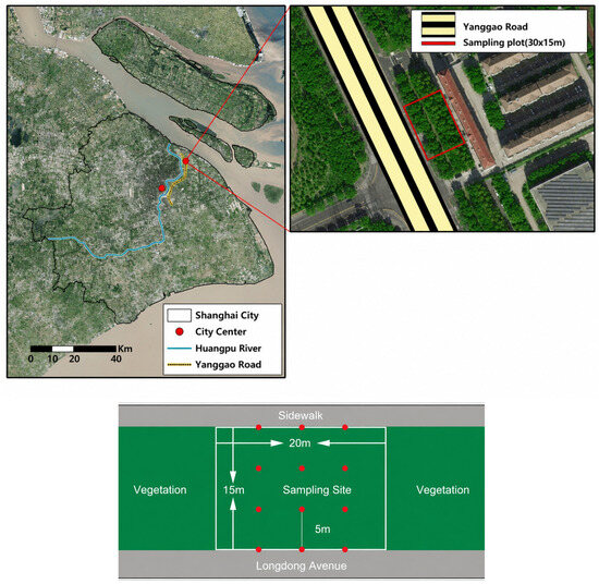
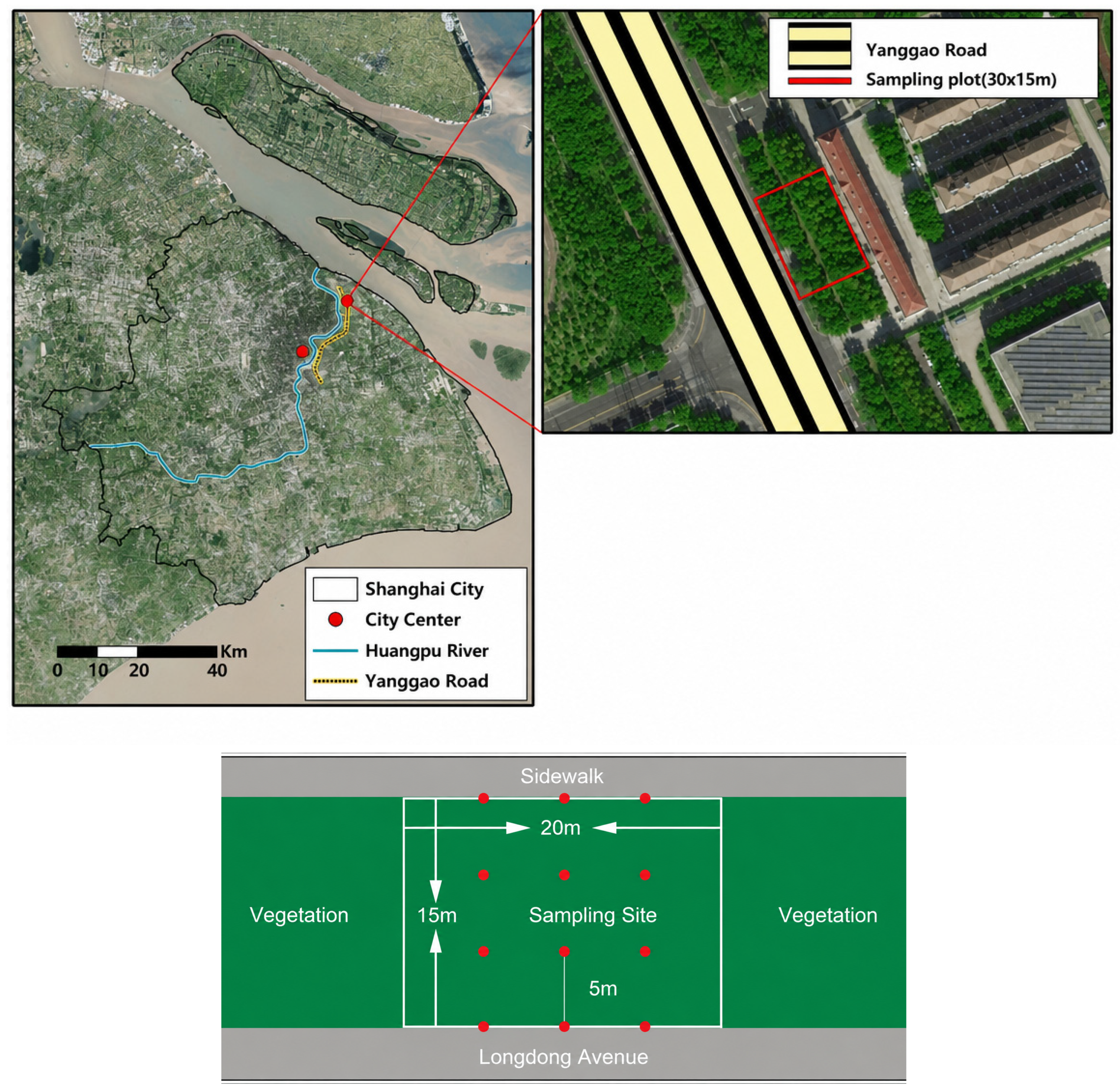
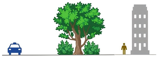
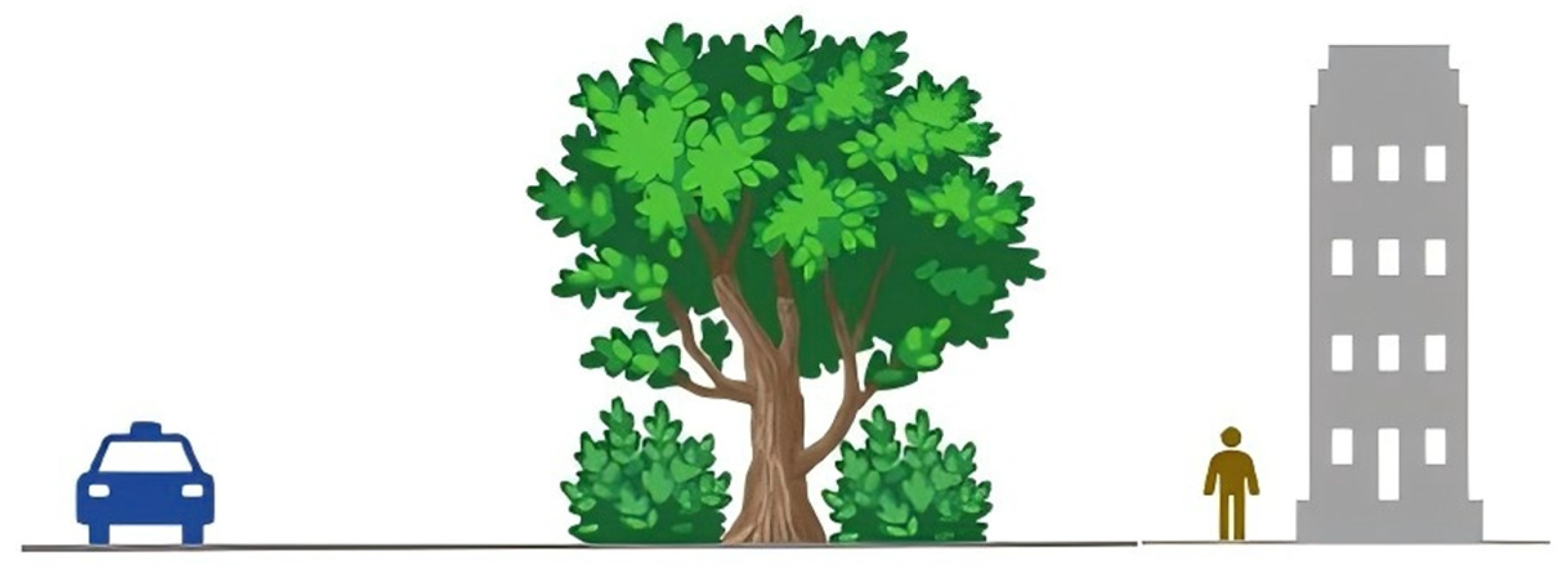
A sample plot with an area of 30 m × 15 m was selected on the east side of Yanggao Road (as shown in Figure 1), and on-site plant species survey and mapping were conducted on this plot. The plants in this sample plot include trees, shrubs and herbs, which can reflect the common plant planting configurations in open road environments in Shanghai. After field investigation, the surface of the area is mainly covered by sparse herbaceous plants, while oleander trees constitute the secondary vegetation layer. In addition, trees of different sizes grow in the area, which together form a green barrier between road traffic and buildings, as shown in Figure 2. Table 2 below shows the distribution of plant species in the sample plots:

Figure 1. Vegetation planting on Yanggao Road.

Figure 2. Open road environment.

Table 2. Plant species statistics.

Plant Name	Type	Quantity	Height (m)	Branch Point Height (m)
Camphor	arbor	8	10.0 × 2 10.6 × 3 9.4 × 3	1.6 × 3 1.8 × 2 2.0 × 3
Yiyang	arbor	2	7.8 × 1 8.2 × 1	1.8 × 2
Oleander	tall shrub	8	5.1 × 2 5.4 × 3 4.6 × 3	/
lawn	Grass	/	0.2–0.3	/

3. Numerical Simulation

Turbulence numerical simulation methods can be divided into direct numerical simulation methods (Direct Numerical Simulation, DNS for short) and indirect numerical simulation methods. The direct numerical simulation method can reproduce the turbulent flow process [12], but its memory space and calculation speed requirements are too high and its use is not considered. Non-numerical simulation methods are also called Large Eddy Simulation (LES), Reynolds-Averaged Navier–Stokes (RANS) and statistical averaging methods. Commonly used non-numerical simulation methods are LES and RANS. Although LES is more accurate than RANS in calculating turbulent motion, its calculation time is too long and it is difficult to refine the inlet conditions and boundary conditions [13]. Therefore, this article uses RANS for simulation.

When using RANS, a Reynolds stress term will be added to the NS equation after homogenization. Two ideas for solving the Reynolds stress term are the Reynolds Stress Model (RSM) and the eddy viscosity model. The eddy viscosity model can be divided into 0-equation, 1-equation and 2-equation models according to different solution methods. The standard k-model is currently the most mature 2-equation model and is widely used in urban neighborhood simulation [14,15].

D. Mumovic et al. [16] studied the sensitivity of six different turbulence models using numerical results of urban street environment simulation and found that the RNGk-model can well simulate the wind environment of buildings on both sides of the road. According to Mumovic’s description, the RNGk-model has built-in corrections, which are applicable in both high and low Reynolds number regions. When the wind speed is higher, the simulation results of the RNGk-model are more accurate.

To sum up, this study will use the RNGk-model as the turbulence model, the RNG k-ε model was selected over the standard k-ε model because it incorporates built-in corrections for low-Reynolds-number regions and provides more accurate predictions of flow separation around bluff bodies, as demonstrated in previous street canyon studies. A steady-state solver was employed because the primary interest of this study is the time-averaged CO₂ concentration field under constant meteorological conditions, which allows efficient comparison of the relative performance of different vegetation configurations. The logarithmic wind profile follows the standard atmospheric boundary layer formulation recommended by Richards and Norris, with a roughness length z₀ = 2 m appropriate for the urban center of Shanghai, and its governing equation is as follows:

Mass conservation equation:

$${\displaystyle \frac{\partial u_i}{\partial x_i}}=0$$

Momentum equation and heat transfer equation:

$${\mathit{u}}_{\mathit{j}}{\displaystyle \frac{\mathsf{\partial }{\mathit{u}}_{\mathit{i}}}{\mathsf{\partial }{\mathit{x}}_{\mathit{j}}}}=-{\displaystyle \frac{\mathbf{1}}{\mathit{\rho }}}{\displaystyle \frac{\mathsf{\partial }\mathit{p}}{\mathsf{\partial }{\mathit{x}}_{\mathit{i}}}}+{\displaystyle \frac{\mathsf{\partial }}{\mathsf{\partial }{\mathit{x}}_{\mathit{j}}}}(\mathit{\vartheta }{\displaystyle \frac{\mathsf{\partial }{\mathit{u}}_{\mathit{i}}}{\mathsf{\partial }{\mathit{x}}_{\mathit{j}}}}-\overline{{\mathit{u}}_{\mathit{i}}^{\mathbf{\prime }}{\mathit{u}}_{\mathit{j}}^{\mathbf{\prime }}})+({\displaystyle \frac{\mathit{\rho }-{\mathit{\rho }}_0}{{\mathit{\rho }}_0}})\mathit{g}$$

$${\mathit{u}}_{\mathit{i}}{\displaystyle \frac{\mathsf{\partial }\mathit{T}}{\mathsf{\partial }{\mathit{x}}_{\mathit{i}}}}+{\displaystyle \frac{\mathsf{\partial }}{\mathsf{\partial }{\mathit{x}}_{\mathit{i}}}}\overline{{\mathit{u}}_{\mathit{i}}^{\mathbf{\prime }}{\mathit{T}}^{\mathbf{\prime }}}={\mathit{S}}_{\mathit{h}}$$

Transfer equations for turbulent kinetic energy (k) and dissipation rate ($\mathsf{\epsilon }$):

$${\mathit{u}}_{\mathit{i}}{\displaystyle \frac{\mathsf{\partial }}{\mathsf{\partial }{\mathit{x}}_{\mathit{i}}}}\mathit{k}={\displaystyle \frac{\mathbf{1}}{\mathit{\rho }}}{\displaystyle \frac{\mathsf{\partial }}{\mathsf{\partial }{\mathit{x}}_{\mathit{j}}}}[{\mathit{\alpha }}_{\mathit{k}}{\mathit{\mu }}_{\mathit{e}\mathit{f}\mathit{f}}{\displaystyle \frac{\mathsf{\partial }\mathit{k}}{\mathsf{\partial }{\mathit{x}}_{\mathit{j}}}}]+{\displaystyle \frac{\mathbf{1}}{\mathit{\rho }}}{\mathit{G}}_{\mathit{k}}+{\displaystyle \frac{\mathbf{1}}{\mathit{\rho }}}{\mathit{G}}_{\mathit{b}}-\mathit{\epsilon }$$

$${\mathit{u}}_{\mathit{i}}{\displaystyle \frac{\mathsf{\partial }}{\mathsf{\partial }{\mathit{x}}_{\mathit{i}}}}\mathit{\epsilon }={\displaystyle \frac{\mathbf{1}}{\mathit{\rho }}}{\displaystyle \frac{\mathsf{\partial }}{\mathsf{\partial }{\mathit{x}}_{\mathit{j}}}}[{\mathit{\alpha }}_{\mathit{\epsilon }}{\mathit{\mu }}_{\mathit{e}\mathit{f}\mathit{f}}{\displaystyle \frac{\mathsf{\partial }\mathit{\epsilon }}{\mathsf{\partial }{\mathit{x}}_{\mathit{j}}}}]+{\mathit{C}}_{\mathbf{1}\mathit{\epsilon }}{\displaystyle \frac{\mathit{\epsilon }}{\mathit{\rho }\mathit{k}}}({\mathit{G}}_{\mathit{k}}+{\mathit{C}}_{\mathbf{3}\mathit{\epsilon }}{\mathit{G}}_{\mathit{b}})-{\mathit{C}}_{\mathbf{2}\mathit{\epsilon }}{\displaystyle \frac{{\mathit{\epsilon }}^{\mathbf{2}}}{\mathit{k}}}$$

Turbulent kinetic energy generation term due to mean velocity gradient (${\mathbf{G}}_{\mathbf{k}}$) and buoyancy (${\mathbf{G}}_{\mathbf{b}}$):

$${\mathit{G}}_{\mathit{k}}={\mathit{\mu }}_{\mathit{t}}{\displaystyle \frac{\mathsf{\partial }{\mathit{u}}_{\mathit{i}}}{\mathsf{\partial }{\mathit{x}}_{\mathit{j}}}}({\displaystyle \frac{\mathsf{\partial }{\mathit{u}}_{\mathit{i}}}{\mathsf{\partial }{\mathit{x}}_{\mathit{j}}}}+{\displaystyle \frac{\mathsf{\partial }{\mathit{u}}_{\mathit{j}}}{\mathsf{\partial }{\mathit{x}}_{\mathit{i}}}})$$

$${\mathit{G}}_{\mathit{b}}=\mathit{g}\mathit{\beta }{\displaystyle \frac{{\mathit{\mu }}_{\mathit{t}}}{\mathit{P}{\mathit{r}}_{\mathit{t}}}}{\displaystyle \frac{\mathsf{\partial }\mathit{T}}{\mathsf{\partial }{\mathit{x}}_{\mathit{i}}}}$$

Thermal expansion coefficient ($\mathsf{\beta }$) and eddy viscosity (${\mathsf{\mu }}_{\mathbf{t}}$):

$$\mathit{\beta }=-{\displaystyle \frac{\mathbf{1}}{\mathit{\rho }}}({\displaystyle \frac{\mathsf{\partial }\mathit{\rho }}{\mathsf{\partial }\mathit{T}}}{)}_{\mathit{P}}$$

$${\mathit{\mu }}_{\mathit{t}}={\displaystyle \frac{\mathit{\rho }{\mathit{C}}_{\mathit{\mu }}{\mathit{k}}^2}{\mathit{\epsilon }}}$$

Herein, $u_i$ and $u_j$ are the time-averaged velocity components in the $\mathit{i}$ and $\mathrm{j}$-directions, respectively (i,j = 1, 2, 3); ${\mu }_{eff}$ is the effective viscosity; $\mathrm{Pr}$ is the turbulent Prandtl number; $P$, $\rho$, and $T$ represent the time-averaged pressure, density, and temperature, respectively; $g$ is the gravitational acceleration; and $S_h$ is the heat source.

$$C_{\mu }=0.0845,{\alpha }_k=1.393,{\alpha }_{\epsilon }=1.393,C_{1\mathit{\epsilon }}=1.42,C_{2\epsilon }=1.68.$$

The momentum equations are solved using the Boussinesq approximation [17]:

$$\rho ={\rho }_0(1-\beta (T-T_0))$$

Herein, ${\rho }_0$ denotes the reference density, $T_0$ denotes the reference temperature, and $\beta$ is the thermal expansion coefficient, which is taken as 0.0033 in this study.

To reduce computational resources, a steady-state solution will be used in this study.

3.1. Physical Model Simplification

This simulation adopted a modular simulation method and carefully constructed the vegetation configuration method of the three-dimensional plant community structure. In view of the extremely lush vegetation in the study area, we chose a modular simulation method that can accurately reflect the efficiency of vegetation in absorbing carbon dioxide, which fully meets the needs of the simulation scenarios set in this study. Empirical evidence shows that trunk volume has a very limited impact on airflow dispersion [18]; therefore only the tree canopy above the average CBH (1.8 m in this study) was included in the study, whereas for shrubs and lawns, the structure from the ground to the top of the individual plant was the object of study. The aerodynamic effect of vegetation was modeled as a porous medium with pressure loss described by the Forchheimer equation. Based on literature values [18], the following porosity (ε) and drag coefficient (Cd) were assigned: for tree canopies, ε = 0.98 and Cd = 0.2; for shrubs, ε = 0.95 and Cd = 0.4; for grass, ε = 0.99 and Cd = 0.1. The canopy height of trees was set to 8 m on average, with a crown diameter of 5 m, based on field measurements listed in Table 2.

3.2. Calculation Area and Grid Setting

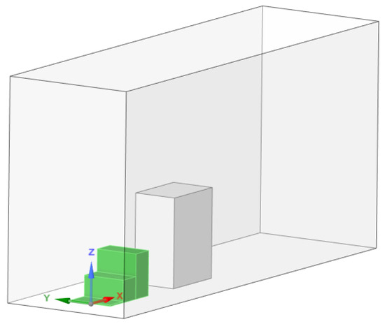
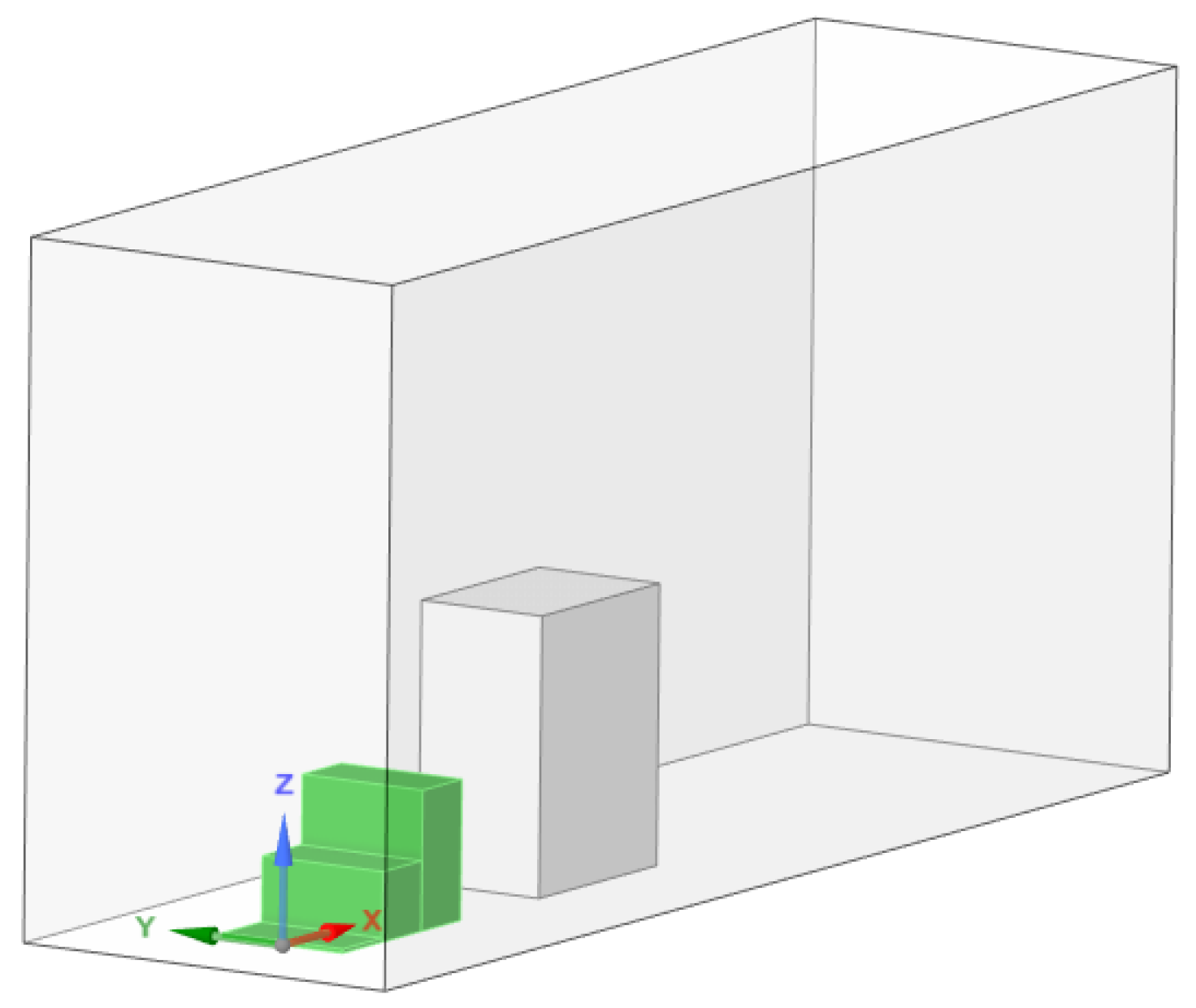
The calculation domain is the space area used for modeling and simulation solutions. In order to solve the discretized fluid flow equation, we need to convert it into a computational grid (or grid). The size of the calculation area will affect the calculation speed and simulation accuracy. If the calculation area is too small, the simulation accuracy will be insufficient, and if the calculation area is too large, it will cause unnecessary waste of computing resources. Referring to the existing research setting [11], the computational domain setting of this study is shown in Figure 3. The distance between plant communities and buildings is 10 m from the lateral boundary and the entrance boundary, and 50 m from the exit boundary. The height of the calculation domain is 50 m.

Figure 3. Three-dimensional computational domain model.

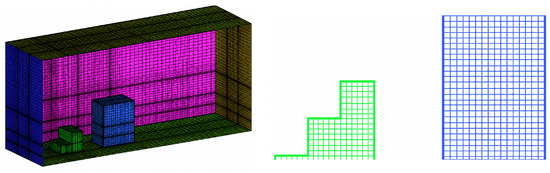
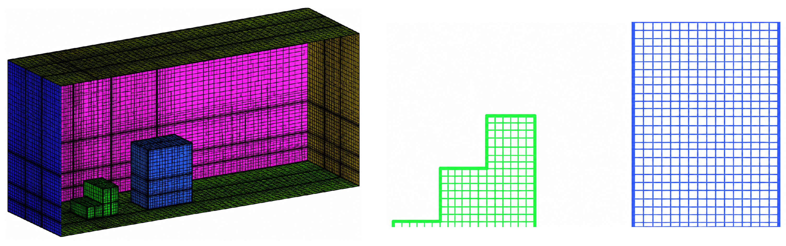
Grid division can spatially discretize the computational domain. Different grid division methods will affect the simulation speed and solution accuracy. Reasonable grid division can improve calculation efficiency and convergence accuracy. The grid types of CFD can be divided into three types: the structured grid, unstructured grid and hybrid grid. The structured grid is established based on the Cartesian coordinate system and is widely recognized and applicable because of its fast generation speed, high calculation accuracy, and relatively good grid quality. The unstructured grid can be applied to some areas with complex spatial shapes, but the calculation time is long. The hybrid grid is a grid type in which structured grids and unstructured grids coexist. The advantage of hybrid grids is that complex geometries can be divided into multiple areas, and unstructured grids are only used in more complex areas to maximize computational efficiency while ensuring accuracy. In summary, the plants and buildings in this study have relatively regular shapes and are suitable for structured grids. The grid division diagram is shown in Figure 4.

Figure 4. Schematic diagram of mesh division. (left) Mesh division diagram; (right) mesh division diagram (XZ plane).

3.3. Boundary Conditions

3.3.1. Inlet Wind Speed Distribution

When the airflow flows through terrain with different characteristics, the energy of the airflow will be reduced due to friction, reducing the wind speed, thus affecting the wind flow field. The degree of this influence will decrease with the increase in height. When reaching a certain height, the roughness of the ground model can be ignored. This height area affected by the surface friction of the earth is called the atmospheric boundary layer. The ambient wind speed is an important boundary condition variable in this study. Research by Pengyi Cui et al. [19] shows that under different environmental wind speed conditions, the wind field structure in streets and alleys will change dramatically. In order to make the simulation results more accurate and closer to the real value, we must consider the change in wind speed with height. Urban environmental wind mainly exists in the form of gradient wind. There are usually two ways to set the gradient wind, usually logarithmic function form and power function form.

In this study, a logarithmic law-based specification of the incoming wind field is adopted. The profiles of mean wind speed (${\mathbf{U}}_{\mathbf{Z}}$), turbulent kinetic energy (${\mathbf{k}}_{\mathbf{Z}}$), and turbulent dissipation rate (${\mathsf{\epsilon }}_{\mathbf{Z}}$) are given as follows [20]:

$${\mathit{U}}_{\mathit{z}}={\displaystyle \frac{{\mathit{U}}_{\mathit{A}\mathit{B}\mathit{L}}^{\mathbf{*}}}{\mathit{\kappa }}}\mathbf{l}\mathbf{n}({\displaystyle \frac{\mathit{z}+{\mathit{z}}_{\mathbf{0}}}{\mathit{z}}})$$

$${\mathit{k}}_{\mathit{z}}={\displaystyle \frac{{\mathit{U}}_{\mathit{A}\mathit{B}\mathit{L}}^{\mathbf{*}}}{\sqrt{{\mathit{C}}_{\mathit{\mu }}}}}$$

$${\mathit{\epsilon }}_{\mathit{Z}}={\displaystyle \frac{{\mathit{U}}_{\mathit{A}\mathit{B}\mathit{L}}^{\mathbf{*}}}{\mathit{\kappa }(\mathit{z}+{\mathit{z}}_{\mathbf{0}})}}$$

where $U_{ABL}^{*}$ is the friction velocity of the atmospheric boundary layer, which can be determined by substituting the wind speed at a given height into the above equations; $\kappa$ is the von Kármán constant, typically taken as 0.4; $z_0$ is the aerodynamic roughness length, whose value depends on the average aerodynamic roughness of the underlying surface within a certain upstream fetch of the incoming wind, and is usually set to 2 m [21] in urban central areas; and $C_{\mu }$ is a constant taken as 0.09.

3.3.2. Outlet Boundary Condition Setting

The fluid flow on the outflow surface of the flow field has been fully diffused, and the flow shape has returned to the flow characteristics without the influence of buildings. Therefore, the outlet boundary is set to the pressure outlet, the pressure at the outlet boundary is set to 0, and the return temperature is equal to the air temperature.

3.3.3. Other Boundary Conditions

Before starting the simulation, in addition to the two key parameters of inlet velocity and outlet pressure, several other parameters are needed to ensure the accuracy and stability of the simulation. First of all, gravity is an indispensable parameter that is necessary for calculations. In addition, several environmental parameters must be provided, including wind direction, air temperature, and carbon dioxide volume fraction. In this study, the real-time average temperature (26 °C) and average carbon dioxide volume fraction (3.96 × 10⁻⁴) measured on site were used and regarded as constants that do not change with altitude. During the fieldwork, the wind direction was a constant easterly.

3.4. Validity Verification

Validity verification is a key step to verify the accuracy of numerical simulation. The validity verification of this study is divided into two parts, namely grid independence verification and field experiment comparison verification. The purpose of the grid independence test is to find the appropriate number of grids and the minimum grid size, while the field experiment comparison verification is to verify whether the simulation settings can restore the real environment.

3.4.1. Grid Independence Test

Grid independence test means to calculate the same model with finer grid division until the grid independence is satisfied when the calculation results are basically unchanged.

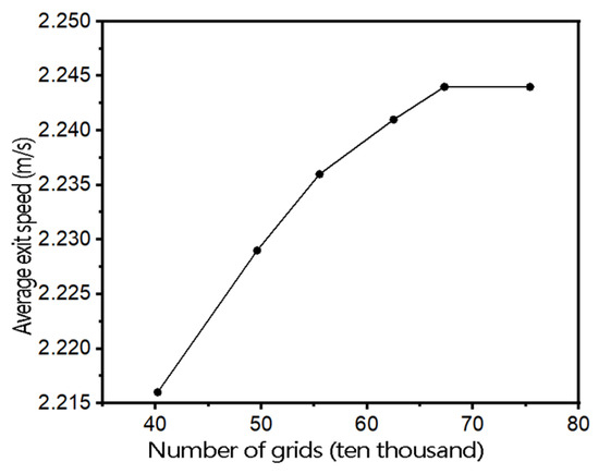
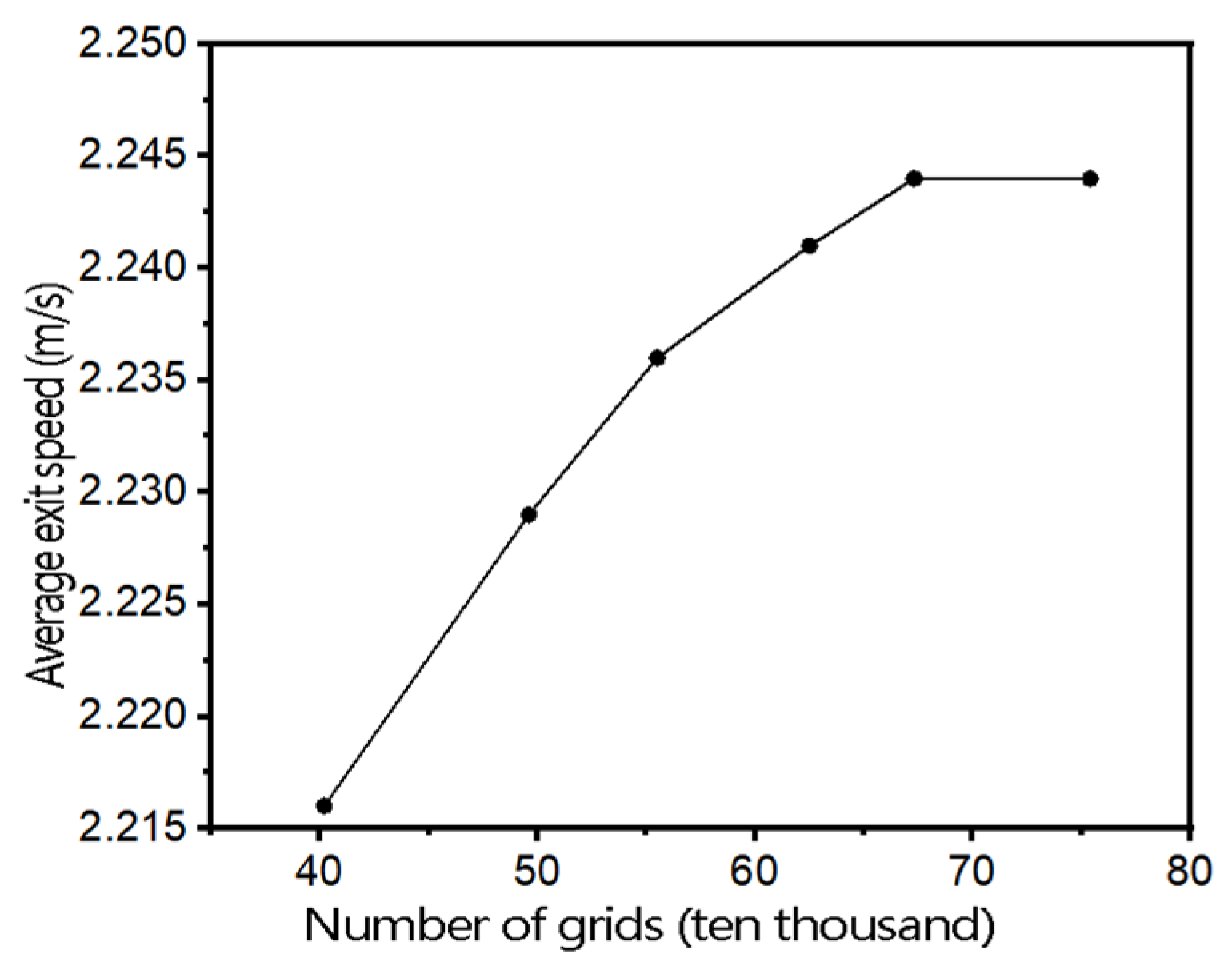
Therefore, before the simulation, in order to eliminate the influence of the number of grids on the accuracy of numerical calculations, the grid independence of the model was verified, and the inlet and outlet pressure drops were calculated under different grid numbers. The flow fields were simulated when the number of grids was 402,000, 496,000, 555,000, 625,000, 673,000 and 754,000 respectively. Taking the average exit speed as an indicator, the average exit speed value under each number of grids is quantitatively analyzed to judge the sensitivity of this numerical simulation to the number of grids.

The grid independence data is shown in Figure 5. According to the calculation results, it can be seen that for different grid numbers, the average outlet speed will change. Within a certain range of the number of grids, the average exit speed increases as the number of grids increases, and then remains stable, with little change after the number of grids reaches 673,000. It can be considered that when the number of grids reaches more than 673,000, the export speed basically becomes consistent. Considering that too many grids will increase the calculation time, this numerical simulation was conducted with 673,000 grids.

Figure 5. The impact of the number of grids on the average exit speed.

3.4.2. Comparison and Verification of Field Experiments

We verified the effectiveness of the three-dimensional computational domain model by comparing the simulated carbon dioxide concentration and wind speed with the actual measured values on site. The simulated CO₂ concentrations and wind speeds were compared with field measurements at 10 sampling points within the study area. The following statistical metrics were used: fractional bias (FB), normalized mean square error (NMSE), and fraction of predictions within a factor of two of observations (FAC2). For CO₂ concentration, FB = 0.08, NMSE = 0.12, and FAC2 = 0.94. For wind speed, FB = 0.10, NMSE = 0.15, and FAC2 = 0.91. These values satisfy common acceptance criteria (|FB| ≤ 0.3, NMSE ≤ 1.5, FAC2 ≥ 0.5) according to Chang and Hanna (2004) [22], confirming that the model is sufficiently accurate for the purpose of comparing vegetation configurations. A sensitivity analysis on inlet wind speed (±20%) and vegetation porosity (±10%) showed that the CO₂ concentration at the building facade changed by less than ±8%, confirming the robustness of the model predictions and the ranking of the six configurations.

3.5. Simulation Scenario

This time, simulation scenarios of six plant community combinations were simulated (Table 3) to evaluate their impact on carbon dioxide distribution in the open road environment in Shanghai urban area. Before conducting the simulation, we processed the plant community block (30 m × 15 m) according to the following steps: First, the block was divided into three parallel planting grooves, each with a size of 30 m × 5 m. The basis for this setting is that plant community combinations with a width of at least 5 m have been proven to be effective in reducing air pollution near roads [23]. Then, different plant types (trees, shrubs, herbs) were planted in each planting tank. When conducting simulations, we made some reasonable approximations and assumptions, mainly including:

(1)

The wind direction blowing from Yanggao Road to the plant communities and buildings is vertical.

(2)

The vegetation planting in each planting slot is continuous and has a rectangular shape.

(3)

For different simulation scenarios, all settings and parameters remain consistent.

Table 3. Plant community combination scene construction.

Simulation Scenario	Planting Mix
	0–5 m	5–10 m	10–15 m
1	arbor	shrub	grass
2	arbor	grass	shrub
3	shrub	arbor	grass
4	shrub	grass	arbor
5	grass	arbor	shrub
6	grass	shrub	arbor

Table 3. Plant community combination scene construction.

Simulation Scenario	Planting Mix
	0–5 m	5–10 m	10–15 m
1	arbor	shrub	grass
2	arbor	grass	shrub
3	shrub	arbor	grass
4	shrub	grass	arbor
5	grass	arbor	shrub
6	grass	shrub	arbor

These simulation scenarios are constructed based on the actual conditions of open road environmental measurements in urban Shanghai and cities in China that also adopt the National Urban Planning and Construction Management Regulations.

4. Conclusions

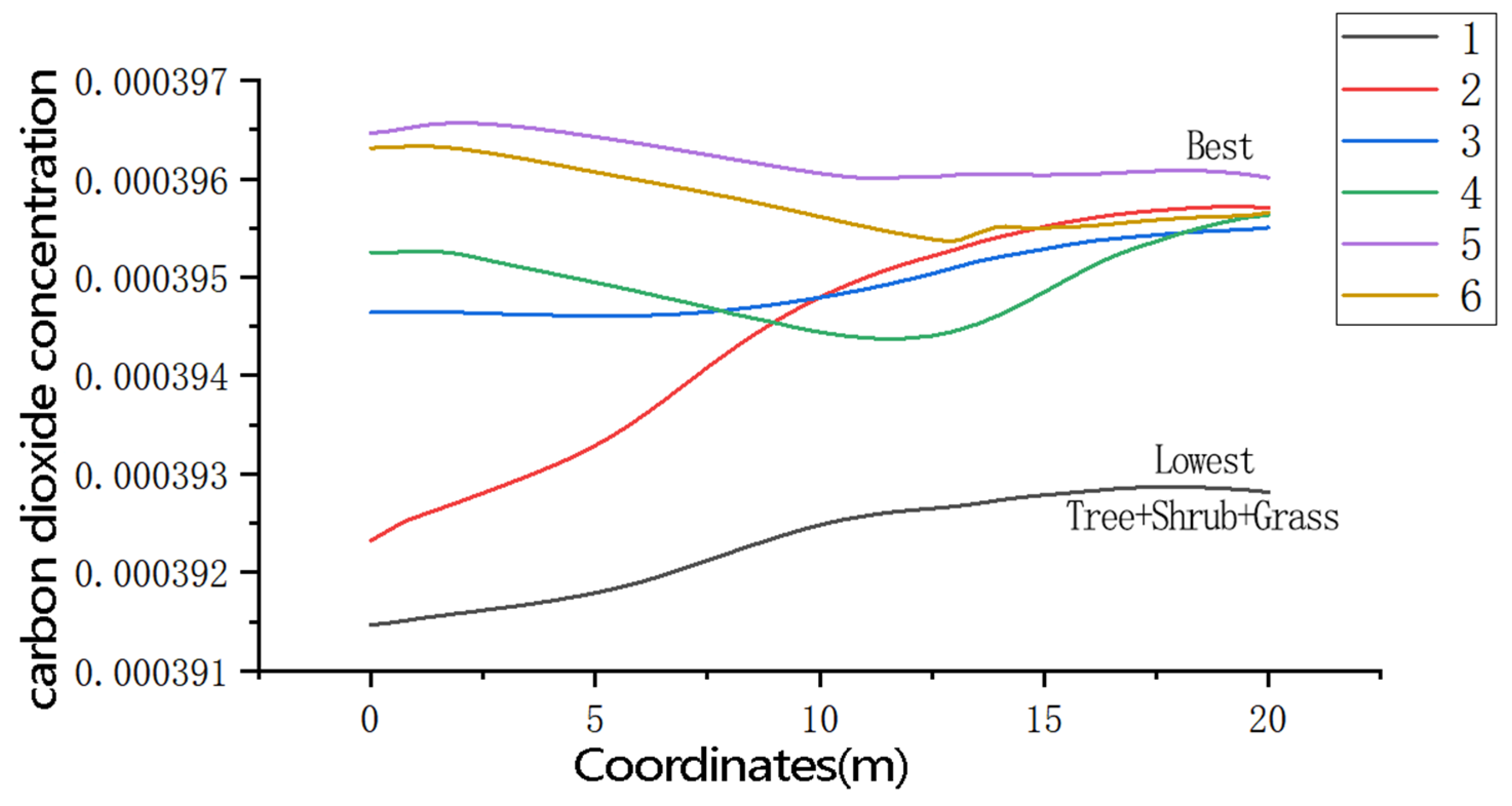
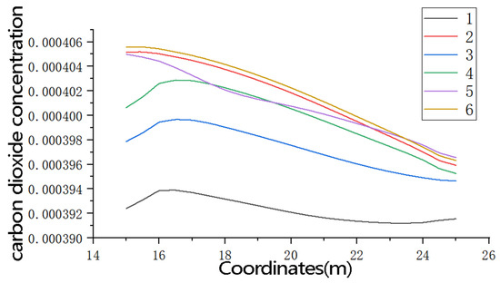
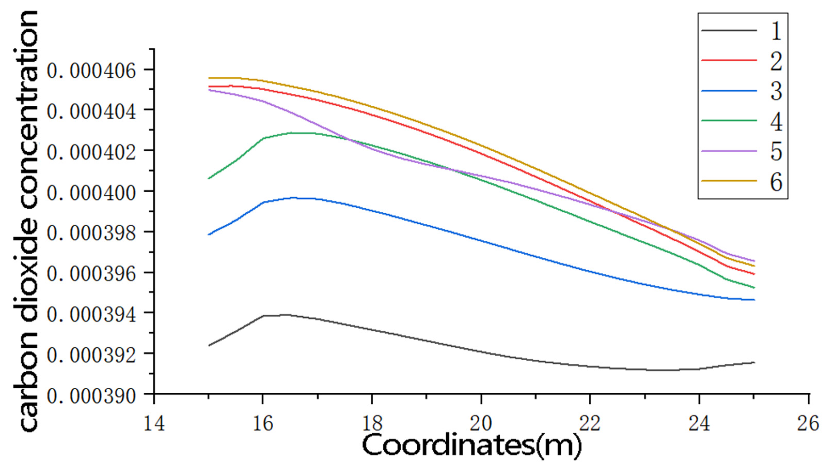
In the calculation of the difference in carbon dioxide concentration directly in front of and behind the plant community, it was found that the plant community has a significant adsorption effect on carbon dioxide. Overall, the introduction of plant communities can effectively reduce carbon dioxide concentrations between plants and buildings, thereby reducing the impact of pollution on both sides of open roads to sidewalk users and residents around buildings. Further analysis of these data revealed that the adsorption of carbon dioxide by plant communities is closely related to plant species and community structure. At a height of 1.5 m from the plant to the building, the tree–shrub–grass combination has the lowest carbon dioxide concentration, indicating that it has the best adsorption effect, with a specific value of 0.000392. This result can be visually observed as shown in Figure 6.

Figure 6. CO₂ concentration at 1.5 m height under six vegetation configurations. The tree–shrub–grass configuration (Scenario 1) exhibits the lowest concentration (3.92 × 10⁻⁴ volume fraction), approximately 12% lower than the highest among the six configurations (Scenario 4). The horizontal dashed line indicates the background CO₂ level measured in the field (3.96 × 10⁻⁴).

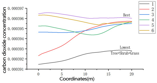
In addition to carbon dioxide reduction, rational allocation of plant community structure also has multiple other advantages, such as reducing traffic noise, reducing PM_2.5 concentration, controlling the urban heat island effect, and reducing runoff. The study by Ferrini et al. in 2020 confirmed this [24]. The distribution of carbon dioxide concentration along the vertical height of the building facade is shown in Figure 7. It can be seen from Figure 7 that for different plant community configurations, the carbon dioxide concentration is different along the height direction of the building. The combination of trees–shrubs–grass has the lowest carbon dioxide concentration, indicating that it has the best adsorption effect. Comparison with previous studies reveals both consistency and novelty. Our finding that a multi-layer vegetation configuration (tree–shrub–grass) outperforms single-layer configurations agrees with Ferrini et al. [24], who reported that mixed vegetation types enhanced pollutant removal. However, unlike previous CFD studies that focused on lateral vegetation belts, our work demonstrates that the longitudinal order of vegetation types along the wind path also matters, with the tree–shrub–grass sequence producing the best performance among the six tested arrangements.

Figure 7. Carbon dioxide concentration distribution along building height.

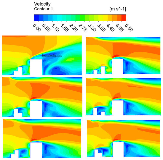
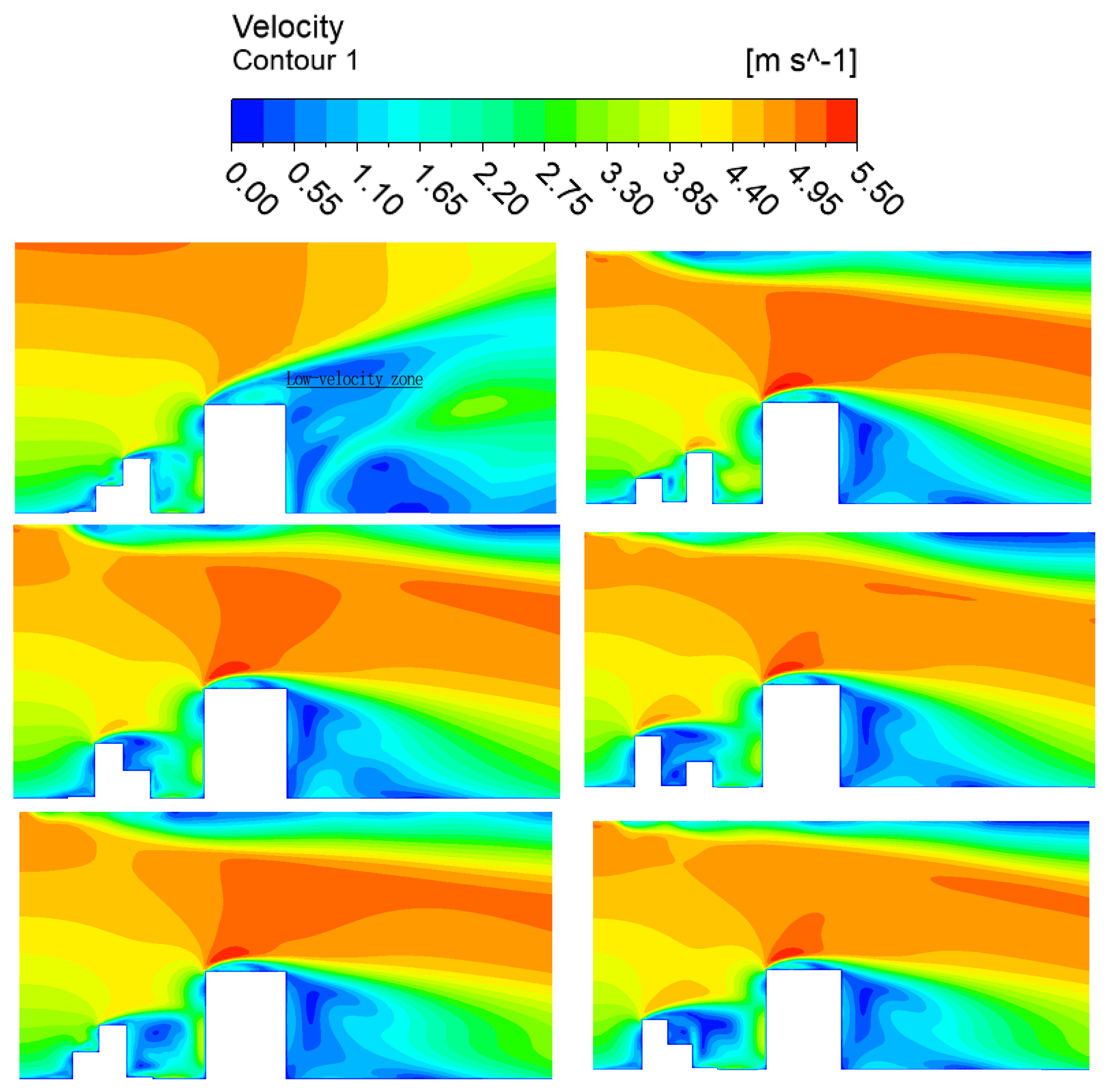
The flow rate has an important influence on the adsorption capacity of carbon dioxide. Figure 8 shows the intermediate cross-sectional velocity distribution under six working conditions. Looking at Figure 8, we can see that the tree–shrub–grass plant community forms a lower velocity area above the building. This phenomenon shows that this plant configuration has a strong adsorption capacity for carbon dioxide.

Figure 8. Speed cloud chart.

Velocity contours (m s⁻¹) on the central vertical cross-section (x–z plane) for the six vegetation configurations. In the tree–shrub–grass configuration (Scenario 1, bottom-right panel), a low-velocity zone forms above the building (indicated by the dark blue region), which enhances local residence time and pollutant deposition. Other configurations show more disrupted flow patterns with higher velocities near the building facade.

This study has limitations that should be addressed in future work. First, only the physical effects of vegetation (flow modification) were modeled; photosynthetic CO₂ uptake would further reduce concentrations, especially during daytime. Second, only one wind direction and summer conditions were simulated; different seasons or wind speeds may alter dispersion patterns. Third, only CO₂ was examined; traffic emits PM_2.5, NOx, and VOCs, which may respond differently to vegetation barriers. Despite these limitations, the present findings provide a useful basis for optimizing roadside vegetation layouts.

References

- Lim, S.; Lee, K.T. Implementation of biofuels in Malaysian transportation sector towards sustainable development: A case study of international cooperation between Malaysia and Japan. Renew. Sustain. Energy Rev. 2012, 16, 1790–1800. [Google Scholar] [CrossRef]
- Timilsina, G.R.; Shrestha, A. Transport sector CO2 emissions growth in Asia: Underlying factors and policy options. Energy Policy 2009, 37, 4523–4539. [Google Scholar] [CrossRef]
- Gasparatos, A.; El-Haram, M.; Horner, M. A longitudinal analysis of the UK transport sector, 1970–2010. Energy Policy 2009, 37, 623–632. [Google Scholar] [CrossRef]
- Muijser, H.; van Triel, J.J.; Duistermaat, E.; Bos, P.M.J. Acute toxicity of high concentrations of carbon dioxide in rats. Regul. Toxicol. Pharmacol. 2014, 69, 201–206. [Google Scholar] [CrossRef]
- Lansing, R.W.; Im, B.S.; Thwing, J.I.; Legedza, A.T.; Banzett, R.B. The perception of respiratory work and effort can be independent of the perception of air hunger. Am. J. Respir. Crit. Care Med. 2000, 162, 1690–1696. [Google Scholar] [CrossRef]
- Jeong, N.; Han, S.; Kim, J. Evaluation of Vegetation Configuration Models for Managing Particulate Matter along the Urban Street Environment. Forests 2022, 13, 46. [Google Scholar] [CrossRef]
- Weissert, L.F.; Salmond, J.A.; Turnbull, J.C.; Schwendenmann, L. Temporal variability in the sources and fluxes of CO2 in a residential area in an evergreen subtropical city. Atmos. Environ. 2016, 143, 164–176. [Google Scholar] [CrossRef]
- Keenan, T.F.; Williams, C.A. The Terrestrial Carbon Sink. Annu. Rev. Environ. Resour. 2018, 43, 219–243. [Google Scholar] [CrossRef]
- Issakhov, A.; Tursynzhanova, A.; Abylkassymova, A. Numerical study of air pollution exposure in idealized urban street canyons: Porous and solid barriers. Urban Clim. 2022, 43, 101112. [Google Scholar] [CrossRef]
- Lateb, M.; Meroney, R.N.; Meroney, M.; Fellouah, H.; Saleh, F.; Boufadel, M.C. On the use of numerical modelling for near-field pollutant dispersion in urban environments − A review. Environ. Pollut. 2016, 208, 271–283. [Google Scholar] [CrossRef]
- Yan, J.; Chen, W.Y.; Zhang, Z.; Zhao, W.; Liu, M.; Yin, S. Mitigating PM2.5 exposure with vegetation barrier and building designs in urban open-road environments based on numerical simulations. Landsc. Urban Plan. 2024, 241, 104918. [Google Scholar] [CrossRef]
- Baglietto, E.; Ninokata, H.; Misawa, T. CFD and DNS methodologies development for fuel bundle simulations. Nucl. Eng. Des. 2006, 236, 1503–1510. [Google Scholar] [CrossRef]
- Sha, C.; Wang, X.; Lin, Y.; Fan, Y.; Chen, X.; Hang, J. The impact of urban open space and ‘lift-up’ building design on building intake fraction and daily pollutant exposure in idealized urban models. Sci. Total Environ. 2018, 633, 1314–1328. [Google Scholar] [CrossRef]
- Zhang, Y.; Ou, C.; Chen, L.; Wu, L.; Liu, J.; Wang, X.; Lin, H.; Gao, P.; Hang, J. Numerical studies of passive and reactive pollutant dispersion in high-density urban models with various building densities and height variations. Build. Environ. 2020, 177, 106916. [Google Scholar] [CrossRef]
- Zhang, Y.; Yang, X.; Yang, H.; Zhang, K.; Wang, X.; Luo, Z.; Hang, J.; Zhou, S. Numerical investigations of reactive pollutant dispersion and personal exposure in 3D urban-like models. Build. Environ. 2020, 169, 106569. [Google Scholar] [CrossRef]
- Mumovic, D.; Crowther, J.M.; Stevanovic, Z. The Effect of Turbulence Models on Numerical Prediction of Air Flow within Street Canyons. In Proceedings of the First International Conference on Computational Mechanics (CM’04), Belgrade, Serbia, 15–17 November 2004. [Google Scholar]
- Zhang, K.; Chen, G.; Zhang, Y.; Liu, S.; Wang, X.; Wang, B.; Hang, J. Integrated impacts of turbulent mixing and NOX-O3 photochemistry on reactive pollutant dispersion and intake fraction in shallow and deep street canyons. Sci. Total Environ. 2020, 712, 135553. [Google Scholar] [CrossRef]
- Yang, H.; Chen, T.; Lin, Y.; Buccolieri, R.; Mattsson, M.; Zhang, M.; Hang, J.; Wang, Q. Integrated impacts of tree planting and street aspect ratios on CO dispersion and personal exposure in full-scale street canyons. Build. Environ. 2020, 169, 106529. [Google Scholar] [CrossRef]
- Cui, P.; Li, Z.; Tao, W. Wind-tunnel measurements for thermal effects on the air flow and pollutant dispersion through different scale urban areas. Build. Environ. 2016, 97, 137–151. [Google Scholar] [CrossRef]
- Richards, P.J.; Norris, S.E. Appropriate boundary conditions for computational wind engineering models revisited. J. Wind Eng. Ind. Aerodyn. 2011, 99, 257–266. [Google Scholar] [CrossRef]
- Blocken, B.; Stathopoulos, T.; Carmeliet, J. CFD simulation of the atmospheric boundary layer: Wall function problems. Atmos. Environ. 2007, 41, 238–252. [Google Scholar] [CrossRef]
- Chang, J.C.; Hanna, S.R. Air quality model performance evaluation. Meteorol. Atmos. Phys. 2004, 87, 167–196. [Google Scholar] [CrossRef]
- Yin, S.; Shen, Z.; Zhou, P.; Zou, X.; Che, S.; Wang, W. Quantifying air pollution attenuation within urban parks: An experimental approach in Shanghai, China. Environ. Pollut. 2011, 159, 2155–2163. [Google Scholar] [CrossRef] [PubMed]
- Ferrini, F.; Fini, A.; Mori, J.; Gori, A. Role of Vegetation as a Mitigating Factor in the Urban Context. Sustainability 2020, 12, 4247. [Google Scholar] [CrossRef]
Disclaimer/Publisher’s Note: The statements, opinions and data contained in all publications are solely those of the individual author(s) and contributor(s) and not of MDPI and/or the editor(s). MDPI and/or the editor(s) disclaim responsibility for any injury to people or property resulting from any ideas, methods, instructions or products referred to in the content. |
© 2026 by the authors. Licensee MDPI, Basel, Switzerland. This article is an open access article distributed under the terms and conditions of the Creative Commons Attribution (CC BY) license.