MFD-DF: A PM_2.5 Concentration Prediction Method Based on Multimodal Feature Decomposition and Dynamic Fusion

Abstract

Accurate air pollutant concentration prediction is crucial for public health and sustainable urban development. Existing methods predominantly rely on single-modal data, resulting in inadequate representation of pollutant spatiotemporal evolution, poor prediction accuracy, and limited generalization capabilities. To address these challenges, this research proposes a novel PM_2.5 prediction framework termed MFD-DF that integrates ground-station time series and satellite remote sensing images. In feature extraction, learnable decomposition and deformable convolution are introduced, and a Cross-Modal Slot Attention module explicitly decomposes features to resolve information blurring. Subsequently, a dynamic cross-modal alignment mechanism is designed alongside a learnable Time-Expansion Network (TEN) to ensure fine-grained interaction. Furthermore, a local-global attention feature fusion mechanism is proposed to optimize data integration efficacy. Experimental results demonstrate that in single-step PM_2.5 prediction tasks, the proposed MFD-DF achieves significant improvements of approximately 10–20% in MAE, RMSE, and MAPE compared to state-of-the-art baselines. In multi-step PM_2.5 prediction, it effectively alleviates the error accumulation problem in long-sequence forecasting, demonstrating superior robustness and accuracy.

1. Introduction

Air pollution is a critical threat to public health and poses profound implications for sustainable urban development [1]. High-concentration accumulation areas frequently overlap with densely populated zones, significantly amplifying population exposure risks [2,3]. Among various atmospheric pollutants, fine particulate matter (PM_2.5) is recognized as one of the most hazardous due to its minute particle size, prolonged atmospheric residence time, and capacity to penetrate pulmonary alveoli into the systemic circulation. The fluctuations in PM_2.5, concentration are governed by a complex interplay of anthropogenic emissions, meteorological conditions, topography, and regional transport. Characterized by pronounced temporal variability, spatial heterogeneity, and multi-source complexity, PM_2.5 dynamics are difficult to capture through monitoring networks alone, which often fail to reflect the rapid evolution of pollution events [4,5]. High-precision prediction provides a scientific foundation for proactive emission reduction, optimized traffic management, and emergency intervention, thereby playing a pivotal role in public health alerts, environmental regulation, and urban planning [6].

With the proliferation of big data and artificial intelligence, traditional statistical modeling has been progressively superseded by deep learning architectures [7,8]. These advanced models have demonstrated superior performance in capturing the temporal evolution and long-range dependencies inherent in PM_2.5 concentrations [9,10]. Nevertheless, a significant proportion of existing approaches remains reliant on single datasets [11,12]. By failing to effectively integrate external driving factors, these models often exhibit insufficient predictive accuracy and limited generalization capabilities when confronted with complex environmental scenarios [13].

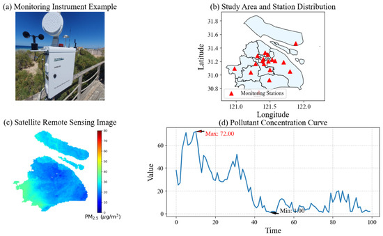
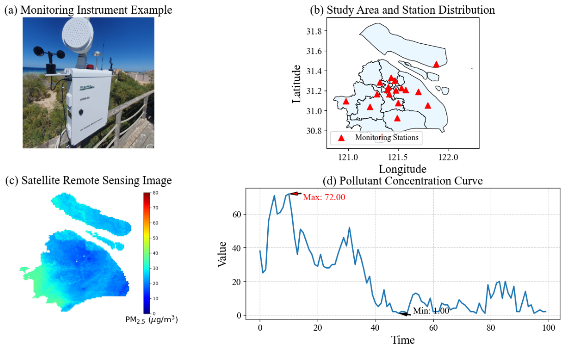
To overcome the constraints of unimodal methods, multimodal data fusion has emerged as a cornerstone of dynamic PM_2.5 prediction. As shown in Figure 1, this study integrates multi-source heterogeneous observational data to enhance characterization capabilities. Point-source time-series data from ground-based sensors provide high-fidelity reflections of localized concentration fluctuations, whereas remote sensing imagery reveals broader spatial distribution and transport characteristics. These two data sources exhibit fundamental spatio-temporal complementarity [14,15]. Integrating these heterogeneous modalities enables the expansion of spatial observation coverage and enhances temporal continuity, yielding a more comprehensive characterization of dispersion processes [16]. However, existing multimodal fusion frameworks encounter several persistent challenges: Differences in temporal resolution and spatial scales across modalities can cause feature misalignment; ambiguous boundaries between shared and modality-specific features lead to information redundancy or leakage; inadequate cross-modal alignment mechanisms limit model stability and generalization performance under complex meteorological conditions [17,18,19,20].

Figure 1. Overview of the study area and examples of multimodal data sources. (a) Actual view of ground-based air quality monitoring equipment; (b) Study area (Shanghai) and spatial distribution of monitoring stations; (c) Example satellite remote sensing imagery of the corresponding area; (d) Time-series variation curves of pollutant concentrations recorded at monitoring stations.

To address the aforementioned issues, this study proposes a multimodal deep learning framework for air quality prediction that integrates time series data with remote sensing imagery. This framework combines time series data from ground monitoring stations with remote sensing image data, incorporating four core modules: feature learning and modeling, feature decomposition and separation, dynamic alignment and deep fusion, and prediction. It effectively integrates multi-source data to capture the spatiotemporal characteristics of air quality changes. Specifically, the innovations of this study include: (1) A dual-path spatiotemporal collaborative learning mechanism is established, employing learnable decomposition and deformable convolutions to capture the non-stationary temporal evolution and irregular spatial diffusion patterns of PM_2.5. This approach resolves the challenge of characterising complex spatiotemporal patterns within heterogeneous datasets. (2) An intra-modal feature decomposition mechanism is established by applying Cross-Modal Slot Attention within each modality to extract shared and modality-specific features, thereby enhancing the complementarity and interpretability of cross-modal fusion. (3) The introduction of the learnable Time-Expansion Network (TEN): By employing dual-transposed convolution technology, TEN dynamically adjusts low-frequency remote sensing features to align with high-frequency time series. This mechanism fine-grained alignment under causal constraints, resolving temporal scale mismatch. (4) A local-global attention mechanism is applied to fuse dimensional information, complemented by adaptive mapping and residual enhancement structures to enhance the model’s predictive accuracy and generalization capability.

The remainder of this paper is organized as follows: Section 2 reviews prior work; Section 3 details the network architecture and loss design of our framework; Section 4 presents the dataset, experimental setup, results, ablation studies, and interpretability analysis; Section 5 concludes the paper and discusses limitations and future work.

2. Related Work

2.1. Air Quality Forecasting

Deep learning-based methods have become the mainstream approach for air quality prediction. Models such as RNN, LSTM, and GRU overcome the limitations of traditional statistical methods by automatically capturing complex dependencies within time series [21,22]. Subsequent research introduced TCN, leveraging dilated convolutions to enhance parallel processing capabilities and performance for long sequences [23]. Transformer-based improvements like Informer, Autoformer, and FEDformer achieved breakthroughs in long-term dependencies and prediction accuracy through attention mechanisms and decomposable modeling [24,25,26]. Models such as AirQFormer further validated this architecture’s immense potential for regional prediction [27,28,29]. Concurrently, modeling spatial correlations is crucial for capturing interactions between monitoring stations and pollutant dispersion. CNN, ST-ConvNet, and graph neural networks like GCN, GAT, and STGCN are widely applied to model topological relationships between stations [30,31]. For instance, E-STGCN enhances robustness during extreme pollution events by integrating extremal theory [32], while AQ-Net improves prediction accuracy for unobserved stations through multi-head attention and spatial interpolation strategies [33]. These advancements collectively establish a deep learning prediction system that evolves from time-dependent to spatiotemporal collaborative modeling.

Despite significant progress in spatiotemporal modeling, existing methods predominantly rely on single-modal data such as time series or images [34]. This limitation hinders the integration of rich information from heterogeneous sources, constraining models’ ability to characterize pollutant evolution and interactions among multiple environmental factors [35]. To address this, this study proposes a multimodal deep learning framework that comprehensively models spatial correlations and spatiotemporal dependencies by deeply integrating time series and remote sensing image data. This approach effectively overcomes the limitations of single-modal information, significantly enhancing the accuracy and robustness of air quality prediction.

2.2. Multimodal Data Fusion Methods

Multimodal data fusion effectively compensates for the limitations of single-modal approaches in spatial coverage and feature representation by integrating information from heterogeneous sources, significantly enhancing model robustness in complex spatiotemporal tasks. In air quality prediction, time series, remote sensing imagery, and meteorological data exhibit high complementarity, facilitating more precise characterization of pollutant formation and evolution [36]. Currently, the deep integration of temporal numerical data with graph/image data has become mainstream. For instance, Res-GCN achieves high-performance multi-step prediction by fusing remote sensing images and station data through ResNet and graph convolutional networks [37]; the FuXi-Air model integrates weather forecasts and emission inventories, balancing accuracy and efficiency in city-level predictions [38]. Furthermore, multimodal dynamic modeling approaches leverage combinations of CNN, Bi-LSTM, and graph networks to effectively capture the spatiotemporal co-evolution of pollutants [39]. Meanwhile, STMFNet enhances the interpretability of cross-modal fusion through a shared-specific feature decomposition mechanism [40].

Although multimodal fusion can effectively enhance accuracy, significant challenges persist in the practical application of PM_2.5 prediction. The frequency alignment mechanism between remote sensing imagery data and station concentration sequences remains imperfect, while incomplete feature decomposition limits the model’s generalisation capability in complex geographical environments and under rapidly changing weather conditions. Furthermore, the model’s limitations in explaining pollutant transport mechanisms and its robustness when confronted with data gaps require further enhancement. Consequently, establishing a fusion mechanism capable of accurately modeling the spatiotemporal evolution of PM_2.5 while maintaining physical interpretability represents the current critical imperative.

3. Methodology

3.1. Overall Framework

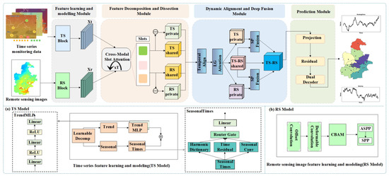
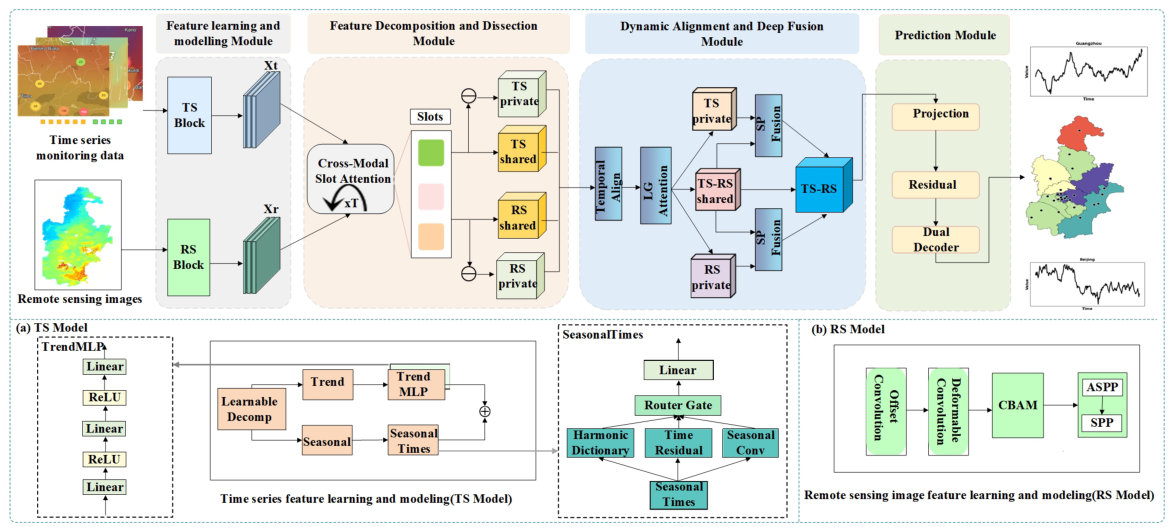
The proposed multimodal air quality prediction framework, as illustrated in Figure 2, comprises four distinct stages. Stage One: Feature Learning. This stage leverages learnable decompositions to capture temporal trends and seasonal patterns within the data. Concurrently, the remote sensing branch employs deformable convolutions and multi-scale attention mechanisms to capture irregular spatial features. Stage Two: Feature Decomposition. Cross-Modal Slot Attention maps heterogeneous features into a unified latent space, explicitly decomposing them into shared and modality-specific components to enhance feature complementarity and eliminate modal redundancy. Stage Three: Dynamic Alignment and Deep Fusion. A Time-Expansion Network (TEN) is constructed, employing dual-transposed convolutions to extend low-frequency remote sensing features to high-frequency scales under causal constraints, resolving temporal resolution mismatches. Subsequently, local-global attention achieves efficient cross-dimensional information fusion. Stage Four: Prediction Output. Employing multi-layer linear mapping coupled with a residual enhancement mechanism, the fused features are transformed into future prediction values. A dual-layer decoder architecture ensures the smoothness and robustness of long-sequence predictions.

Figure 2. Overall Framework diagram of proposed model.

3.2. Time Series Feature Learning and Modeling

To accurately model the complex evolution patterns within air quality data, this study introduces two dimensions: long-term trends and seasonal cycles. The former reflects persistent fluctuations in pollutants arising from policy interventions or macro-environmental shifts, while the latter characterises recurring patterns influenced by meteorological conditions, diurnal variations, and human activities. This study proposes a learnable decomposition module that splits the time series $x_t\in {\mathbb{R}}^{B\times L\times N}$ into trend components ${\widehat{t}}_t$ and seasonal components ${\widehat{s}}_t$. To accommodate localized spatiotemporal heterogeneities, input data is sampled via sliding windows with an adaptive lookback length ($L_{\mathrm{lookback}}$). Specifically, $L_{\mathrm{lookback}}$ is set to 96 h for Beijing to capture prolonged pollutant accumulation across its 34 stations, and 48 h for Tianjin, Shanghai, and Guangzhou to cover two complete 24-h diurnal emission cycles. This differentiated setting optimizes the temporal receptive field for multi-scale feature learning. This module employs one-dimensional convolutional layers (Conv1d) to extract deep features along the temporal axis and smooth short-term fluctuations. Unlike traditional statistical decomposition, this mechanism adaptively fits regional data distributions via backpropagation, significantly enhancing the representation of non-stationarity in PM_2.5 dynamic evolution.

$${\widehat{t}}_t=Conv1d\left(ReLU\left(BN\left(Conv1d\left(x_t\right)\right)\right)\right)$$

(1)

$${\widehat{s}}_t=x_t-{\widehat{t}}_t$$

(2)

In the trend modeling section, we employ the TrendMLPBlock for non-linear reconstruction of trend sequences. This module comprises a three-layer feedforward network. TrendMLP performs non-linear mappings on the sequence dimension of trend components, enabling the model to learn more flexible trend representations beyond the constraints of traditional linear trend modeling.

$${\widehat{t}}_t^{\mathrm{out}}=\mathrm{TrendMLP}\left({\widehat{t}}_t\right).$$

(3)

Seasonal variation does not follow a single pattern but is instead composed of regular cyclical components, irregular local fluctuations, and slow seasonal residuals. To address this, the SeasonalTimesBlock module is employed to construct a three-branch seasonal modeling structure. By dynamically integrating these three feature types through a router, the model can adaptively select the optimal seasonal representation for each time period, significantly enhancing the expressiveness of seasonal components and the stability of forecasts. Firstly, a sparse harmonic dictionary is utilised to extract seasonal features.

$${\widehat{s}}_t^{\mathrm{dict}}=Dict\_Proj\left(Softshrink\left(Encoder\left({\widehat{s}}_t\right)\right)\right)$$

(4)

Among these, Encoder(${\widehat{s}}_t$) encodes the input data, obtaining sparse encoding coefficients via the Softshrink function. Here, Dict_Proj performs the operation of mapping sparse encoding coefficients to a higher-dimensional space, yielding seasonal features. Secondly, temporal residual features are extracted by mapping the input data to a new feature space.

$${\widehat{s}}_t^{\mathrm{res}}=ToD\left({\widehat{s}}_t\right)$$

(5)

Among these, ToD is a linear transformation process that maps inputs to a new space, with the resulting features capturing temporal correlations and dynamic changes within time series. To further capture more complex seasonal fluctuations, convolutional operations can model seasonal variation patterns through local awareness, particularly for non-sinusoidal seasonal variations.

$${\widehat{s}}_t^{\mathrm{conv}}=Conv\left({\widehat{s}}_t\right)$$

(6)

The gate mechanism dynamically adjusts feature weights, integrating sparse harmonic dictionary features ${\widehat{s}}_t^{\mathrm{dict}}$, temporal residual features ${\widehat{s}}_t^{\mathrm{res}}$, and convolutional features ${\widehat{s}}_t^{\mathrm{conv}}$. The modelled seasonal sequence is output as follows:

$${\widehat{s}}_t^{\mathrm{out}}={\widehat{s}}_t^{\mathrm{dict}}·{\omega }_{\mathrm{dict}}+{\widehat{s}}_t^{\mathrm{res}}·{\omega }_{\mathrm{res}}+{\widehat{s}}_t^{\mathrm{conv}}·{\omega }_{\mathrm{conv}}.$$

(7)

Finally, we derive trend component features and seasonal component features respectively from two independent time series feature extraction branches. These are then combined to yield the final time series features.

$$X_t={\widehat{t}}_t^{\mathrm{out}}+{\widehat{s}}_t^{\mathrm{out}}$$

(8)

3.3. Remote Sensing Image Feature Learning and Modeling Module

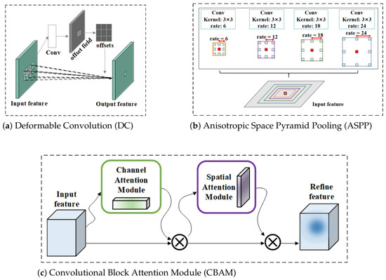
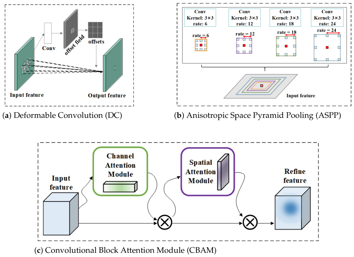
To characterize the spatial distribution and environmental heterogeneity of PM_2.5, this study developed a multi-scale feature extractor integrating Deformable Convolution (DC), ASPP, and CBAM. Its core logic involves: utilizing ASPP’s multi-rate hollow convolution to capture cross-regional diffusion patterns, while employing CBAM to focus on key pollution sources and suppress background noise across spatial and channel dimensions.

Given that traditional convolutions are constrained by fixed geometric structures and struggle to characterize the irregular evolution of PM_2.5 plumes, this study introduces DC to enhance spatial modeling flexibility. For input remote sensing images $I\in {\mathbb{R}}^{B\times C\times H\times W}$, where $L_r$, this module adapts sampling criteria to irregular pollutant morphologies through learnable offsets $\Delta p$. The feature extraction process of DC can be expressed as:

$$F_{\mathrm{def}}\left(p_0\right)=\sum _{p\in \mathcal{R}}\omega \left(p\right)·I(p_0+p+\Delta p),$$

(9)

Here, p denotes the center coordinate, and R defines the sampling range of the standard convolution kernel. By introducing an offset, the model can more accurately fit spatial patterns under complex meteorological conditions, significantly enhancing feature robustness in heterogeneous environments. To enhance salient region features, CBAM is introduced. Figure 3 illustrates the detailed structural workflow of CBAM. First, the channel attention module weights image features to compute global average pooling and max pooling results in the channel dimension.

$$M_c\left(F\right)=\sigma \left(W_2\delta \left(W_1\mathrm{Avg}\left(F\right)\right)+W_2\delta \left(W_1\mathrm{Max}\left(F\right)\right)\right)$$

(10)

Figure 3. Key Module Architecture for Remote Sensing Image Processing: (a) Deformable Convolution (DC); (b) Anisotropic Space Pyramid Pooling (ASPP); (c) Convolutional Block Attention Module (CBAM).

Here, $\delta (·)$ denotes ReLU and $\sigma (·)$ denotes Sigmoid. Spatial attention is based on average pooling and max pooling along the channel dimension:

$$M_s\left(F\right)=\sigma \left(W_3·[\mathrm{Avg}\left(F\right);\mathrm{Max}\left(F\right)]\right)$$

(11)

$$F_{\mathrm{attn}}=M_s\left(M_c\left(F\right)\odot F\right)$$

(12)

To capture multi-scale spatial patterns, the ASPP module is employed. This module extracts image features at different scales by applying convolutional operations at varying dilation rates. Through multi-scale convolutional operations, we can extract both local and global spatial information from images, which is crucial for enhancing the model’s spatial perception capabilities.

$$F_{\mathrm{aspp}}=\mathrm{Concat}\left(\{{\mathrm{Conv}}_r\left(F_{\mathrm{attn}}\right)\mid r\in \{1,6,12\}\},\mathrm{GP}\left(F_{\mathrm{attn}}\right)\right)$$

(13)

Here, Conv_r denotes convolution with a stringency rate of r, while GP represents global pooling. Simultaneously employing SPP to further capture local-to-global hierarchical features:

$$F_{\mathrm{spp}}=\mathrm{Concat}\left(P_{1\times 1}\left(F_{\mathrm{aspp}}\right),P_{2\times 2}\left(F_{\mathrm{aspp}}\right),P_{3\times 3}\left(F_{\mathrm{aspp}}\right),\mathrm{GP}\left(F_{\mathrm{aspp}}\right)\right)$$

(14)

Finally, the multi-scale features are concatenated and fed into a fully connected layer, mapping them to a unified latent space:

$$Z_{\mathrm{rs}}=\varphi \left(W·[F_{\mathrm{aspp}};F_{\mathrm{spp}}]+b\right),Z_{\mathrm{rs}}\in {\mathbb{R}}^{B\times C\times D}$$

(15)

3.4. Feature Decomposition and Deconstruction Module

In multimodal air quality prediction, remote sensing imagery and time-series data respectively capture macro-spatial patterns and local temporal dynamics. However, these two sources exhibit feature redundancy and coupling. Direct fusion may lead to intermodal information confusion, weakening the expressiveness of shared features and reducing the discernibility of specific information. Therefore, this paper introduces a feature decomposition mechanism. By explicitly separating modal features, it enables more rational cross-modal interaction.

Specifically, given the time-series modal representation $X_t\in {\mathbb{R}}^{B\times N\times D}$ and the remote sensing image modal representation $X_r\in {\mathbb{R}}^{B\times C\times D}$, they are first concatenated into a unified input:

$$X=[X_t;X_r]\in {\mathbb{R}}^{B\times T\times D}$$

(16)

This is achieved through the Cross-Modal Slot Attention mechanism, whose core idea is to utilize a small number of learnable slot vector $S\in {\mathbb{R}}^{S\times D}$ as aggregators for shared feature information. By applying a scaled dot-product attention mechanism, the slot vectors interact with modal tokens to obtain an attention weight matrix A. Where Q is the channel vector, K is the input feature, and D is the feature dimension. Based on attention aggregation, the shared representation is updated as follows.

$${\tilde{X}}_{\mathrm{sh}}=A·S,{\tilde{X}}_{\mathrm{sh}}\in {\mathbb{R}}^{B\times T\times D}$$

(17)

Subsequently, it is decomposed into two components, ${\tilde{X}}_{t\_\mathrm{sh}}$ and ${\tilde{X}}_{r\_\mathrm{sh}}$, and the mode-specific representation is defined in residual form:

$$X_{t\_\mathrm{pv}}=X_t-{\tilde{X}}_{t\_\mathrm{sh}},X_{r\_\mathrm{pv}}=X_r-{\tilde{X}}_{r\_\mathrm{sh}}$$

(18)

To further enhance decomposition performance, this paper introduces three types of regularization constraints during training:

(1) Shared Contrastive Loss ${\mathcal{L}}_{\mathrm{sh}}$, which enhances the expressive power of shared information by aligning cross-modal shared representations ${\tilde{X}}_{t\_\mathrm{sh}}$ and ${\tilde{X}}_{r\_\mathrm{sh}}$, thereby promoting information sharing across different modalities.

$${\mathcal{L}}_{\mathrm{sh}}=-{\displaystyle \frac{1}{B}}{\displaystyle \sum _{i=1}^B}\log \left({\displaystyle \frac{\exp \left({\tilde{X}}_{t\_\mathrm{sh}}^i·{\tilde{X}}_{r\_\mathrm{sh}}^i\right)}{{\sum }_{j=1}^B\exp \left({\tilde{X}}_{t\_\mathrm{sh}}^i·{\tilde{X}}_{r\_\mathrm{sh}}^j\right)}}\right)$$

(19)

(2) Private Disparity Loss ${\mathcal{L}}_{\mathrm{pv}}$, which prevents over-coupling by incentivizing differentiation between private features $X_{t\_\mathrm{pv}}$ and $X_{r\_\mathrm{pv}}$ across different modalities.

$${\mathcal{L}}_{\mathrm{pv}}={\displaystyle \frac{1}{B}}{\displaystyle \sum _{i=1}^B}\left({∥{\displaystyle \frac{X_{t\_\mathrm{pv}}^i·X_{r\_\mathrm{pv}}^i}{\parallel X_{t\_\mathrm{pv}}^i\parallel \parallel X_{r\_\mathrm{pv}}^i\parallel }}∥}^2\right)$$

(20)

(3) Orthogonal Loss ${\mathcal{L}}_{\mathrm{ortho}}$ encourages orthogonality between shared and private features to suppress interference between them.

$${\mathcal{L}}_{\mathrm{ortho}}={\displaystyle \frac{1}{B}}{\displaystyle \sum _{i=1}^B}\left({∥{\tilde{X}}_{t\_\mathrm{sh}}^i·X_{t\_\mathrm{pv}}^i∥}^2+{∥{\tilde{X}}_{r\_\mathrm{sh}}^i·X_{r\_\mathrm{pv}}^i∥}^2\right)$$

(21)

The final decomposition loss is:

$${\mathcal{L}}_{\mathrm{dec}}=\alpha {\mathcal{L}}_{\mathrm{sh}}+\beta {\mathcal{L}}_{\mathrm{pv}}+\gamma {\mathcal{L}}_{\mathrm{ortho}}.$$

(22)

3.5. Dynamic Alignment and Deep Fusion Module

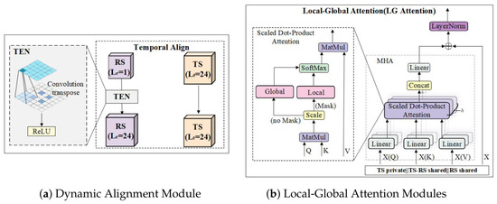
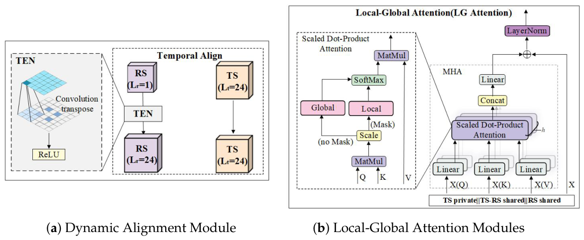
Before multimodal features enter the fusion stage, the disparity in temporal resolution between time series data and remote sensing imagery poses a significant challenge. Specifically, time series data typically exhibit hourly granularity Lt, whereas remote sensing images generally feature daily granularity Lr. This discrepancy results in differing token sequence lengths, hindering direct cross-modal interaction. To address this issue, this paper proposes a learnable Time Expansion Network (TEN). This network employs 1D transposed convolutions to downsample the token sequences of remote sensing images from daily resolution to hourly resolution, thereby achieving temporal alignment between the two modalities. Subsequently, a Dynamic Alignment module is designed to ensure that features from both modalities can interact on a unified temporal scale, thereby enhancing the computational efficiency of the cross-modal attention mechanism.

$$\begin{array}{cc}\hfill X_{r\_\mathrm{pv}}^{\mathrm{align}}& ={\mathrm{TEN}}_{\mathrm{pv}}\left(X_{r\_\mathrm{pv}}\right),{\mathrm{TEN}}_{\mathrm{pv}}\left(X\right)=\mathrm{ReLU}\left({\mathrm{Conv}1\mathrm{D}}_{\mathrm{trans}}^{\mathrm{pv}}\left(X\right)\right)\hfill \end{array}$$

(23)

$$\begin{array}{cc}\hfill X_{r\_\mathrm{sh}}^{\mathrm{align}}& ={\mathrm{TEN}}_{\mathrm{sh}}\left(X_{r\_\mathrm{sh}}\right),{\mathrm{TEN}}_{\mathrm{sh}}\left(X\right)=\mathrm{ReLU}\left({\mathrm{Conv}1\mathrm{D}}_{\mathrm{trans}}^{\mathrm{sh}}\left(X\right)\right)\hfill \end{array}$$

(24)

Subsequently, the aligned shared features from both modalities are concatenated at the sequence dimension to obtain the fused shared feature $X_{\mathrm{sh}}^{\mathrm{align}}$. This is then input alongside the aligned modality-specific features into the cross-modal attention module, enabling deep interaction between multimodal information.

$$X_{sh}^{\mathrm{aligned}}=Concat(X_{t\_sh},X_{r\_sh}^{\mathrm{aligned}})$$

(25)

To effectively fuse multi-modal features, this paper proposes a fusion module comprising two core components: a local-global attention mechanism and a shared-specific gated fusion layer. The local-global attention mechanism employs multi-head attention (MHA) to capture both local and global dependencies among multi-modal features, as illustrated in Figure 4. We first compute the attention weights:

$$\mathrm{Attention}(Q,K,V)=\mathrm{Softmax}\left({\displaystyle \frac{Q{K}^{\top }}{\sqrt{D}}}+M\right)V$$

(26)

Figure 4. Detailed Schematic Diagram of the Dynamic Alignment and Local-Global Attention Module.

Here, M denotes the adjacency mask matrix, employed to constrain local connections thereby achieving a comprehensive modeling of neighbourhood and global relationships. The output undergoes residual connection and layer normalisation:

$$LGAtt\left(X\right)=\mathrm{LayerNorm}(X+\mathrm{Attention}(Q,K,V\left)\right)$$

(27)

Building upon the modeling of local-global relationships, we further designed a gating mechanism to adaptively weight shared representations against specific representations. First, concatenation is performed, and the result is fed into two layers of perceptrons to learn the importance weights of specific features and shared features within the current spatio-temporal region:

$$g=\mathrm{Softmax}(MLP\left([X_{pv};X_{sh}]\right)$$

(28)

Here, $g_{pv}$ and $g_{sh}$ denote the model’s preference for modality-specific information and cross-modality shared information respectively. The fused features are obtained by weighting specific features and shared features according to their respective weights. This gating mechanism automatically adjusts the proportion of specific versus shared information based on pollution characteristics across different times and regions, thereby yielding a more stable and discernible cross-modality fusion representation.

$$X^{\mathrm{fusion}}=g_{\mathrm{pv}}·X_{\mathrm{pv}}+g_{\mathrm{sh}}·X_{\mathrm{sh}}$$

(29)

Unlike traditional methods that fuse only two feature streams, this paper preserves three types of semantically complementary information: time-specific, remote-sensing-specific, and cross-modal shared features. These are then stitched together to form the final fused representation:

$$h_{\mathrm{fusion}}=Concat(X_{\mathrm{t}}^{fusion},X_{\mathrm{sh}},X_{\mathrm{r}}^{fusion})$$

(30)

3.6. Prediction Module

Following cross-modal alignment and fusion, the model acquires a high-dimensional sequence representation incorporating complementary multimodal information. The objective of the prediction module is to map these fused semantic features to the future PM_2.5 concentrations at the monitoring site. To this end, the module employs a prediction architecture comprising feature compression, adaptive mapping, and residual augmentation prediction. To reduce redundancy in the cross-modal fused representation and enhance the discriminative power of features for the prediction task, the fused representation is first compressed using a layer combining linear transformation with a nonlinear activation function:

$$h_1=\sigma (W_1{h}_{fusion}+b_1)$$

(31)

The number of tokens ${\mathrm{L}}_f$ obtained after cross-modal fusion often differs from the number of monitoring stations N, leading to spatial dimension mismatch when performing direct predictions. To address this issue, this paper designs an adaptive mapping mechanism that employs a dynamically generated mapping matrix to map token sequences of arbitrary length to representations of a fixed number of monitoring stations.

$$h_{\mathrm{node}}=\left(W_{map}{h}_1\right),W_{map}\in {\mathbb{R}}^{L_f\times N}$$

(32)

To further enhance the model’s stability for long-term prediction, a residual prediction augmentation structure $h=h_{\mathrm{ts}}+h_{\mathrm{node}}$ is employed. Here, $h_{\mathrm{ts}}$ denotes the high-frequency dynamic features extracted by the time series backbone network, while $h_{\mathrm{node}}$ represents the prediction representation after cross-modal fusion. Finally, the augmented representation is mapped to the target time domain via a two-layer linear decoder to generate PM_2.5 forecast values for the next T steps:

$$h_{\mathrm{dec}}=\sigma (W_{2}h+b_2)$$

(33)

$$Y=W_3{h}_{dec}+b_3$$

(34)

4. Experiment and Result Analysis

4.1. Datasets

This experiment constructed a multimodal dataset integrating ground-based monitoring and remote sensing imagery for four cities: Tianjin, Beijing, Shanghai, and Guangzhou. Time Series Dataset: Data originates from real-time observations recorded at ground-based air quality monitoring stations across each city. This study collected hourly ${\mathrm{PM}}_{2.5}$ concentration values from each station. This dataset features high temporal resolution, enabling precise capture of short-term fluctuations and sudden changes in pollutant concentrations. To secure data integrity and quality assurance before training, a basic preprocessing pipeline was executed: continuous missing records extending under 3 h were filled via temporal linear interpolation, while anomalous negative outliers or tracking artifacts caused by transient sensor telemetry noise were systematically filtered and calibrated using localized historical rolling averages. Remote Sensing Image Dataset: The raw satellite imagery is explicitly sourced from the ChinaHigh${\mathrm{PM}}_{2.5}$ (CHAP) national daily dataset. This high-resolution dataset provides seamless spatio-temporal coverage of ground-level ${\mathrm{PM}}_{2.5}$ concentrations at a spatial resolution of $1\mathrm{km}\times 1\mathrm{km}$ and a daily temporal resolution.

To capture regional pollutant transport, daily images were collected to strictly match the calendar days within each city’s designated observation period: 1096 images for Beijing (a 3-year span including the 2020 leap year), 365 images each for Tianjin and Shanghai (1-year spans), and 366 images for Guangzhou (a 1-year span encompassing the 2024 leap year). These collected multi-temporal images were then spatially clipped using city-level Shapefile vector boundaries and aligned via geographic coordinates. Subsequently, the regional concentration values were mapped to grayscale and uniformly resampled to effectively reflect pollutant transport and dispersion dynamics. The detailed specifications of the integrated datasets are summarized in Table 1.

Table 1. Detailed information of the four datasets.

Datasets	Tianjin	Beijing	Shanghai	Guangzhou
Stations	27	34	18	21
Time Stamps	8760	26,280	8760	8784
Start Date	1 May 2014	1 Janurary 2018	1 Janurary 2022	1 Janurary 2024
End Date	1 May 2015	1 Janurary 2021	1 Janurary 2023	1 Janurary 2025
Time Interval	1 (h)	1 (h)	1 (h)	1 (h)
Data Acquisition Interval	1 (h)	1 (h)	1 (h)	1 (h)
Remote Sensing Images	365	1096	365	366

4.2. Experimental Setup

All experiments were implemented using the Pytorch 2.5.1 framework in a Python 3.10 environment and were implemented using the PyTorch framework within a Python environment and were accelerated by an NVIDIA RTX 4090 GPU. To ensure a fair comparison, all models were evaluated using identical input and output dimensions during the benchmarking phase, while the other hyperparameter configurations for the baselines were set according to the default values specified in their original publications. The proposed framework was trained utilizing the Adam optimizer with a learning rate of $1\times {10}^{-4}$. Additional architectural and training parameters of the proposed model are detailed in Table 2.

Table 2. Detailed hyperparameter settings of preposed model.

Hyperparameter	Tianjin	Beijing	Shanghai	Guangzhou
Learning Rate	$1\times {10}^{-4}$	$1\times {10}^{-4}$	$1\times {10}^{-4}$	$1\times {10}^{-4}$
Optimizer	Adam	Adam	Adam	Adam
Batch Size	32	64	32	32
Patience	5	5	5	5
Feature Dimension	64	96	64	96
Time Window Size	48	96	48	48

4.3. Evaluation Metrics

This experiment employed three commonly used regression model evaluation metrics to assess the performance of the multimodal air quality prediction model: MAE, RMSE, and MAPE.

MAE: The average of the absolute differences between predicted values and actual values. It provides an intuitive assessment method, where smaller values indicate that predictions are closer to actual values.

$$\mathrm{MAE}={\displaystyle \frac{1}{N}}{\displaystyle \sum _{i=1}^N}|y_i-{\widehat{y}}_i|$$

(35)

RMSE: Represents the average of squared errors, where larger errors exert a greater influence on its value. It is suitable for identifying significant errors.

$$\mathrm{RMSE}=\sqrt{{\displaystyle \frac{1}{N}}\sum _{i=1}^N{(y_i-{\widehat{y}}_i)}^2}$$

(36)

MAPE: Calculates the relative error between predicted and actual values, expressed as a percentage. It is suitable for evaluating the relative accuracy of different prediction tasks. A smaller MAPE value indicates higher prediction accuracy.

$$\mathrm{MAPE}={\displaystyle \frac{1}{N}}{\displaystyle \sum _{i=1}^N}\left|{\displaystyle \frac{y_i-{\widehat{y}}_i}{y_i}}\right|\times 100\%$$

(37)

4.4. Analysis of Experimental Results

This section presents experimental results of the multimodal air quality prediction model across various city datasets, comparing it with existing benchmark models. Our approach demonstrates superior performance across multiple city datasets, particularly in short-term prediction tasks. Compared to the state-of-the-art model STMFNet [40], our method achieves significant improvements in MAE, RMSE, and MAPE metrics, indicating its advantage in capturing dynamic changes in air quality.

4.4.1. Single-Step Prediction Results

This section presents experimental results of different methods across multiple urban datasets. Through comparative analysis, we validate the effectiveness of our proposed multimodal air quality prediction approach. Table 3 demonstrates the performance of each model in the single-step prediction task.

Table 3. The single-step prediction performance of Ours and other baselines on four datasets. The best performance is highlighted in bold, while the second-best is underlined.

Methods	Guangzhou-2024				Shanghai-2022				Beijing-2018				Tianjin-2014
	MAE	RMSE	MAPE		MAE	RMSE	MAPE		MAE	RMSE	MAPE		MAE	RMSE	MAPE
LSTM	5.35	7.83	0.18		8.86	14.39	0.38		8.48	13.51	0.43		16.69	25.62	0.37
Transformer	4.96	7.47	0.16		7.62	13.32	0.35		7.07	11.15	0.36		16.80	25.61	0.34
Informer	4.03	5.79	0.13		6.43	11.28	0.32		5.35	8.39	0.31		14.68	22.17	0.30
TimeNet	3.38	4.80	0.12		5.74	9.32	0.29		5.48	8.83	0.33		13.05	19.89	0.29
DLinear	2.61	4.24	0.08		5.47	8.44	0.25		4.58	7.99	0.27		11.40	20.56	0.24
STMFNet	2.77	4.24	0.09		5.00	8.19	0.25		4.50	7.36	0.26		10.09	16.60	0.22
MFD-DF (ours)	2.42	3.90	0.07		4.42	7.33	0.21		4.18	6.99	0.23		8.83	15.60	0.19

In single-step prediction tasks, MFD-DF demonstrates significant improvements compared to the state-of-the-art model STMFNet. Specifically, MFD-DF achieves reductions of 10.83% to 12.49% in MAE, 6.02% to 10.50% in RMSE, and 11.54% to 22.22% in MAPE across Guangzhou, Shanghai, Beijing, and Tianjin. These results demonstrate that through multimodal data fusion, our model achieves substantial gains in accuracy and stability for short-term prediction, enabling it to better capture the spatiotemporal variations in air quality.

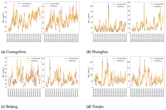
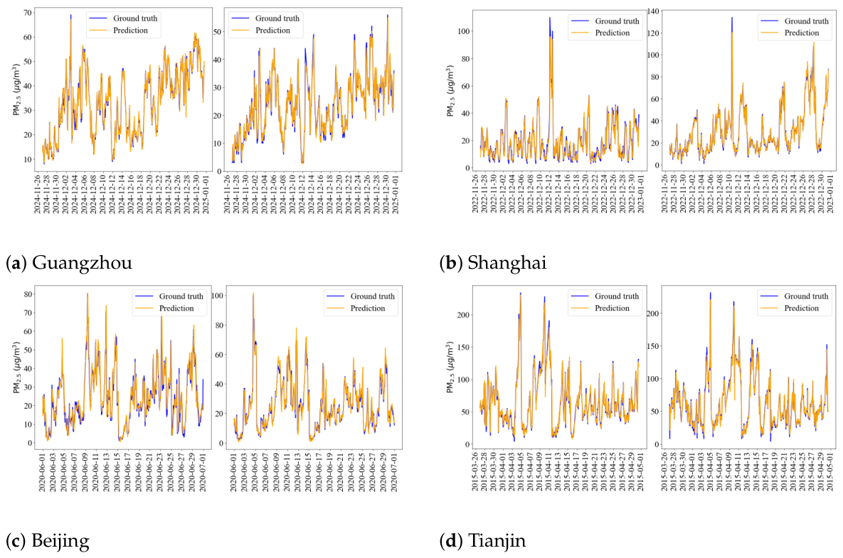
Single-site visualisations demonstrate the comparison between predicted and actual PM_2.5 values over time at various monitoring stations across Guangzhou, Shanghai, Beijing, and Tianjin. As illustrated in Figure 5, we observe the contrast between forecasted and recorded PM_2.5 concentrations at randomly selected stations within each city. The figures clearly demonstrate that the model effectively tracks the long-term trends in air quality data and delivers accurate predictions for the majority of time points. Even during sudden fluctuations or short-term variations, the model continues to reflect data changes with reasonable precision, showcasing its robust predictive capabilities.

Figure 5. Visualization of single-site forecast results for four cities.

4.4.2. Multi-Step Prediction Results

To validate our model’s multi-step prediction capability, we conducted prediction experiments at 12-h, 24-h, 36-h, and 48-h horizons. Table 4 presents the multi-step prediction results for our model across multiple cities, including MAE, RMSE, and MAPE metrics, alongside comparisons with existing benchmark models.

Table 4. Multi-step prediction performance of Ours and other baselines across four datasets. The best performance is highlighted in bold, while the second-best is underlined.

Dataset	Methods	12 h				24 h				36 h				48 h
		MAE	RMSE	MAPE		MAE	RMSE	MAPE		MAE	RMSE	MAPE		MAE	RMSE	MAPE
Tianjin-2014	LSTM	25.72	36.49	0.65		30.67	40.26	0.88		35.33	44.89	1.23		39.95	49.63	1.35
	Transformer	25.43	35.37	0.55		28.07	38.72	0.82		32.60	42.67	0.90		33.95	45.52	0.97
	Informer	24.65	35.52	0.62		27.57	38.15	0.70		28.85	39.07	0.66		30.47	41.12	0.77
	TimeNet	23.05	32.94	0.54		26.57	37.28	0.65		28.72	40.27	0.70		30.21	42.36	0.68
	DLinear	21.31	31.25	0.49		26.31	36.45	0.62		27.87	38.05	0.66		29.67	40.84	0.68
	STMFNet	21.71	30.82	0.51		25.96	35.42	0.64		27.65	37.85	0.66		28.87	39.03	0.70
	MFD-DF (ours)	21.04	30.74	0.43		25.25	35.38	0.59		27.50	37.51	0.64		28.09	38.56	0.66
Beijing-2018	LSTM	14.02	21.36	0.98		18.90	26.89	1.30		20.40	29.45	1.41		22.55	30.47	1.69
	Transformer	13.76	20.94	0.95		17.28	25.13	1.26		18.98	28.12	1.32		20.42	28.88	1.67
	Informer	13.01	20.51	0.79		16.39	24.39	1.23		18.24	28.02	1.24		19.19	28.06	1.45
	TimeNet	12.31	20.09	0.80		16.21	25.36	1.21		18.55	28.64	1.36		20.27	30.45	1.41
	DLinear	12.54	20.38	0.90		15.89	24.19	1.29		17.68	26.11	1.47		18.75	27.06	1.59
	STMFNet	11.64	18.84	0.76		15.34	23.35	1.20		17.01	25.28	1.34		18.12	26.47	1.41
	MFD-DF (ours)	11.10	18.15	0.73		14.79	22.74	1.12		16.70	25.07	1.21		17.97	26.04	1.40
Shanghai-2022	LSTM	17.74	29.92	0.87		20.55	33.99	0.92		22.23	35.07	0.93		24.87	38.34	1.22
	Transformer	17.13	28.30	0.75		19.80	33.12	0.80		21.82	34.31	0.89		20.81	36.50	1.06
	Informer	15.75	25.92	0.76		18.73	29.97	0.88		20.52	31.91	0.97		21.30	33.63	0.97
	TimeNet	13.31	22.33	0.70		16.36	26.80	0.87		18.22	29.70	1.02		19.10	30.61	0.99
	DLinear	12.42	20.83	0.64		15.63	25.87	0.84		17.08	28.18	0.77		17.93	29.76	0.86
	STMFNet	12.35	20.76	0.63		15.48	25.84	0.77		17.05	28.40	0.82		17.87	29.77	0.85
	MFD-DF (ours)	11.88	19.74	0.62		14.84	24.32	0.75		16.79	27.49	0.81		17.72	29.26	0.84
Guangzhou-2024	LSTM	9.41	12.91	0.35		13.25	17.87	0.44		15.40	19.99	0.48		16.19	20.72	0.51
	Transformer	9.17	12.59	0.31		12.62	16.58	0.40		13.89	18.08	0.41		15.12	19.46	0.43
	Informer	10.40	14.15	0.33		12.19	16.05	0.40		14.89	19.36	0.44		14.44	18.81	0.43
	TimeNet	7.80	10.52	0.30		10.28	13.29	0.36		12.42	15.67	0.38		13.58	16.82	0.41
	DLinear	7.75	10.84	0.23		9.68	13.08	0.28		11.05	14.81	0.31		12.06	15.86	0.34
	STMFNet	7.58	10.54	0.24		9.61	12.97	0.29		11.24	14.82	0.34		12.01	15.92	0.36
	MFD-DF (ours)	7.01	10.03	0.20		9.24	12.76	0.27		10.96	14.70	0.30		11.77	15.73	0.33

In multi-step prediction tasks, the MFD-DF model maintains optimal performance across all cities and forecast time steps. Its advantage is particularly pronounced in short-term forecasts. In Beijing and Tianjin, MFD-DF significantly outperforms baseline models on metrics such as MAE. In Guangzhou and Shanghai, the model achieves substantial improvements in prediction accuracy, with average enhancements of 10.87% and 8.24% in MAE and RMSE, respectively. Overall, while performance improvements across all models gradually plateaued over time, MFD-DF consistently maintained optimal results. This strongly demonstrates that multimodal fusion strategies effectively enhance model robustness and stability, with particularly pronounced advantages in short-term prediction—critical for environmental emergency alerts.

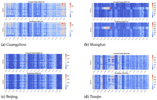
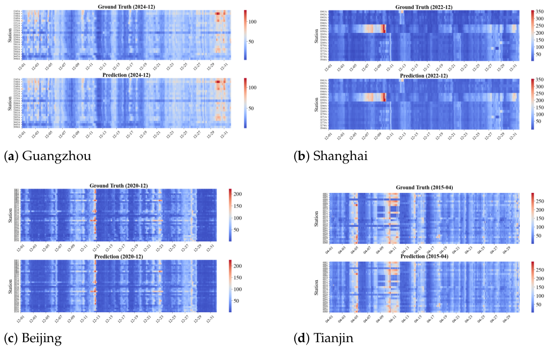
To demonstrate the predictive performance across multiple sites, we selected stations from several cities and visualized the comparison between predicted and actual PM_2.5 values using heatmaps. Figure 6 shows the comparison of predicted versus actual values for stations in Guangzhou, Shanghai, Beijing, and Tianjin. These visualizations allow us to intuitively observe the model’s predictive performance over different time periods, particularly its handling of PM_2.5 concentration changes and short-term fluctuations across various cities. Overall, the proposed model demonstrates excellent capability in capturing trends within time series data, achieving strong fit with actual measurements. Notably, during high-pollution events and short-term fluctuations, the model’s predictions closely align with real values, showcasing robust predictive power. Furthermore, consistent prediction performance across cities highlights the model’s robustness and generalization ability, indicating the framework’s adaptability for cross-city air quality prediction tasks.

Figure 6. Multi-site Visualization of Four Cities.

4.4.3. Spatial Prediction Results

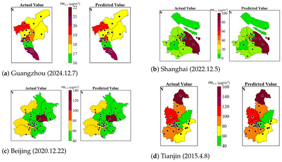
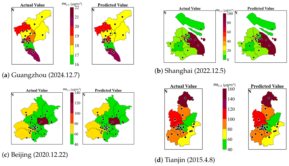
To evaluate the regional prediction performance of the MFD-DF model, we employed an administrative region aggregation approach. Specifically, we calculated the weighted average of the predicted data for each monitoring station based on its corresponding administrative region to obtain regional average PM_2.5 predictions. Subsequently, these regional average prediction maps were compared with the distribution of actual observed values. Figure 7 shows the comparison between actual and predicted values for a randomly selected day across the four cities.

Figure 7. Comparison of predicted and actual PM_2.5 concentration spatial distributions: (a) Guangzhou, (b) Shanghai, (c) Beijing, and (d) Tianjin.

4.5. Ablation Studies

4.5.1. Overall Framework Ablation

To thoroughly analyze the contribution of each module in our proposed model to its overall performance, this section evaluates the role of each key component through a series of ablation experiments. By systematically removing different modules for analysis, we gain clearer insights into the role each part plays in enhancing model performance, thereby providing a basis for subsequent model optimization and improvement.

1. w/o CMSDA: Remove the Cross-Modal Slot Attention Decouple module and process multimodal data using standard concatenation instead, evaluating its contribution to model performance.

2. w/o TAM: Remove the Temporal Alignment module and directly align time series and remote sensing image data to analyze the role of cross-frequency alignment in improving model accuracy.

3. w/o LGAM: Remove the Local-Global Attention Module and adopt a traditional attention mechanism to evaluate the effectiveness of local-global attention in capturing spatio-temporal features.

4. w/o SPFM: Remove the Shared-Specific Modality Fusion module and employ simple concatenation instead to analyze its role in multimodal data fusion.

5. w/o RSD: Remove remote sensing image data and train/predict using only time series data to evaluate the contribution of multimodal data to model performance.

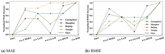
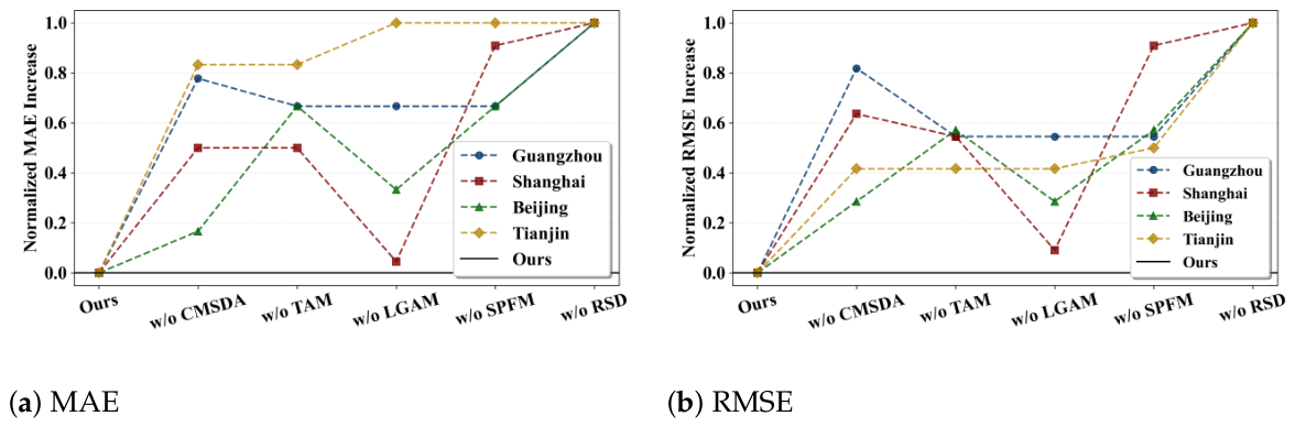
As shown in Figure 8, this paper first normalized the MAE and RMSE experimental results across cities to eliminate the impact of data scale differences between regions, thereby enabling a more objective assessment of each module’s relative contribution to performance improvement. The CMSDA module significantly enhances feature expression capabilities; removing this module degrades model performance, demonstrating the critical role of decomposition mechanisms in multimodal data processing. The TAM module is essential for aligning temporal scales across modalities, particularly in long-step prediction tasks, where its removal leads to a significant drop in model accuracy. The LGAM module enhances the model’s ability to capture complex spatio-temporal dynamics by improving spatio-temporal feature extraction, and its removal markedly reduces model stability. The SPFM module optimizes the fusion effect of multi-modal data, and its removal diminishes both fusion efficiency and accuracy.

Figure 8. Comparison of Ablation Experiment Results for Key Modules of the Overall Framework.

Notably, removing the RSD module had the most severe impact on performance, validating the irreplaceable role of remote sensing imagery in spatio-temporal information extraction. Experiments demonstrate that remote sensing images plays a vital role in long-term prediction tasks for Tianjin and Beijing, particularly in capturing spatio-temporal variations and pollution dispersion. Even in Shanghai and Guangzhou, where environmental changes are relatively stable, removing remote sensing imagery still leads to a decline in model performance, further underscoring its importance in providing spatial information and capturing spatio-temporal dynamics.

4.5.2. Remote Sensing Image Feature Learning and Modeling Dissolution

To further validate the contribution of the remote sensing image feature extraction module to model performance, we conducted ablation experiments to analyze the impact of different feature extraction methods on model effectiveness.

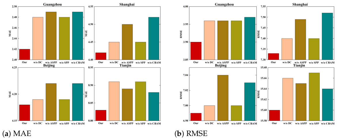
1. w/o DC: The deformable convolution module was removed and replaced with traditional large-kernel convolution for feature extraction from remote sensing images. This ablation experiment verifies the role of deformable convolution in enhancing feature expressiveness.

2. w/o ASPP: The Anisotropic Spatial Pyramid Pooling module was removed, employing conventional convolution operations for feature extraction. This experiment analyzes the role of ASPP in multi-scale feature extraction.

3. w/o SPP: The Spatial Pyramid Pooling module is removed to validate its effect on multi-scale feature aggregation. This experiment evaluates SPP’s influence on enhancing the model’s spatial information representation capability.

4. w/o CBAM: The Channel-Bidirectional Attention Mechanism module was removed, and feature extraction was performed directly using a standard convolutional network. This experiment evaluated the contribution of the CBAM module to feature expressiveness and performance.

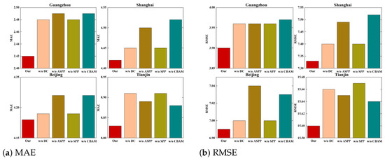
As demonstrated by the ablation results in Figure 9, the DC, ASPP, SPP, and CBAM modules play pivotal roles in enhancing model performance, particularly in feature representation and spatio-temporal information extraction. The DC module is crucial for model performance by strengthening image feature extraction capabilities; its removal leads to a decline in model accuracy. The ASPP and SPP modules significantly improve model robustness and stability through multi-scale feature extraction and spatial information aggregation. Finally, the CBAM module enhances the model’s focus on critical information through its attention mechanism, effectively improving prediction accuracy and stability—especially in long-step prediction tasks. Collectively, these modules significantly strengthen the feature learning and modeling capabilities for remote sensing images, demonstrating their indispensable roles in enhancing overall model performance.

Figure 9. Ablation study results for components within the remote sensing image feature learning and modeling.

4.6. Parameter Sensitivity Analysis

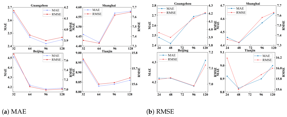
The study conducted a sensitivity analysis of the framework by selecting two key hyperparameters: feature dimension and input time window size. By testing different hyperparameter configurations across four datasets, we visualised MAE and RMSE values for these parameters in single-step prediction tasks, providing an intuitive understanding of their impact on model performance. Specifically, we set the feature dimension to [32, 64, 96, 128] and the time window size to [24, 48, 96, 120]. By comparing single-step prediction errors across different hyperparameter configurations, the analysis results, as illustrated in the figure, demonstrate the impact of varying settings on prediction errors.

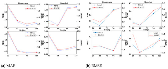
Results for the four cities as observed in Figure 10, moderate feature dimensions and time window sizes effectively enhance the model’s predictive performance. In Guangzhou and Beijing, a feature dimension of 96 yielded optimal results, with prediction errors increasing as the feature dimension grew. Shanghai and Tianjin exhibited divergent trends, with Shanghai and Beijing achieving best performance at a feature dimension of 64. Regarding time windows, all cities exhibited a gradual increase in error as window size expanded. Notably, Guangzhou, Shanghai, and Tianjin achieved optimal prediction at a window size of 48, whereas Beijing performed best at 96. This indicates that selecting appropriate feature dimensions and time windows significantly impacts prediction accuracy. Moderate settings effectively enhance model performance, whereas excessively large or small configurations may lead to deterioration in model capability.

Figure 10. Analysis of Parameter Effects on Model Prediction Errors (MAE and RMSE): (a) Feature Dimension Parameter, (b) Input Time Window Size.

5. Conclusions

Although the compiled datasets deliver rich spatiotemporal trajectories for urban ${\mathrm{PM}}_{2.5}$ tracking, we must acknowledge certain inherent limitations and bound configurations. First, physical data collection governed by hourly and daily sampling granularities is inevitably susceptible to sensor synchronization lags, telemetry dropouts, and subsequent artificial smoothing. Such discrete boundaries can introduce unintended dataset artifacts, including synthetic micro-scale trends or flattened fluctuations. To mitigate over-fitting to these artifacts, our framework strategically deploys a learnable decomposition module with temporal 1D convolutional layers (Conv1d) acting as an adaptive low-pass filter to smooth out transient noise. Second, empirical stress-testing revealed specific marginal conditions where the proposed framework may experience performance degradation. This failure mode primarily manifests during abrupt, non-periodic anthropogenic anomalies or extreme meteorological shocks, such as extensive fireworks during traditional festival eves or sudden catastrophic sandstorms. Under these extreme conditions, the sharp PM_2.5 spikes are heavily driven by stochastic external factors rather than historical evolutionary cycles, causing the model’s trend-seasonal decomposition to exhibit a short-term tracking lag.

This study proposes a multi-modal data fusion framework for air quality prediction. At its core, the model incorporates an information decomposition mechanism to extract shared and private features across modalities. Combined with dynamic alignment and local-global attention mechanisms, it resolves challenges posed by heterogeneous data scales and multi-scale feature representation. Experimental results demonstrate that this approach significantly outperforms mainstream models across multiple urban datasets in metrics such as MAE and RMSE, particularly excelling in capturing transient fluctuations and spatial distribution variations in air quality. Ablation studies further confirm that remote sensing information and the alignment module play a pivotal role in enhancing the model’s robustness and generalisation capability. Future research will explore incorporating higher-frequency meteorological factors and cross-regional transfer learning strategies to enhance the model’s adaptability and predictive accuracy across diverse climatic zones and sparsely monitored regions.

References

- Xia, Y.; McCracken, T.; Liu, T.; Chen, P.; Metcalf, A.; Fan, C. Understanding the Disparities of PM2.5 Air Pollution in Urban Areas via Deep Support Vector Regression. arXiv 2024, arXiv:2405.08416. [Google Scholar]
- Nie, X.; Pan, Y.; Zhang, Y.; Luo, Z.; Wang, S. Battery health prediction under data scarcity: A cross-domain physics-informed 5-shot framework with GRU-Transformer. Appl. Energy 2026, 402, 127012. [Google Scholar] [CrossRef]
- Chen, L.; Liu, T.; Zuo, Z. The health effects of exposure to PM2.5: A review. J. Environ. Health Sci. Eng. 2020, 18, 235–246. [Google Scholar]
- Sorek-Hamer, M.; von Bismarck, M.; Kloog, I.; Cohen, A.J.; Just, A.C.; Broday, D.M. A Deep Learning Approach for Meter-Scale Air Quality Estimation in Urban Environments Using Very High-Spatial-Resolution Satellite Imagery. Atmosphere 2022, 13, 696. [Google Scholar] [CrossRef] [PubMed]
- Wei, J.; Li, Z.; Lyapustin, A.; Sun, L.; Peng, Y.; Xue, W.; Su, T.; Cribb, M.; King, M.D. Full-coverage PM2.5 concentrations at high resolution in China from 2000 to 2021: Space-time model development and applications. Environ. Sci. Technol. 2023, 57, 11136–11147. [Google Scholar]
- Zhang, T.; Wang, X.; Gong, S.; Zhou, Y.; Han, S. Quantifying the impact of meteorological conditions and emission reductions on PM2.5 concentration during the COVID-19 period. Atmos. Environ. 2024, 318, 120253. [Google Scholar] [CrossRef]
- Hassija, V.; Chamola, V.; Mahapatra, A.; Singal, A.; Goel, D.; Huang, K.; Scardapane, S.; Spinelli, I.; Mahmud, M.; Hussain, A. Interpreting Black-Box Models: A Review on Explainable Artificial Intelligence. arXiv 2023, arXiv:2308.00074. [Google Scholar]
- Gu, Y.; Zhao, Y.; Zhou, J.; Li, H.; Wang, Y. A fuzzy multiple linear regression model based on meteorological factors for air quality index forecast. J. Intell. Fuzzy Syst. 2021, 40, 10523–10547. [Google Scholar] [CrossRef]
- Tasan, M.; Ghorbaninasab, Z.; Haji-Aghajany, S.; Ghiasvand, A. Leveraging GNSS tropospheric products for machine learning-based land subsidence prediction. Sci. Rep. 2023, 16, 3056. [Google Scholar] [CrossRef]
- Zhang, Z.; Yang, F. Review of deep learning in air quality prediction. Environ. Model. Softw. 2022, 152, 104426. [Google Scholar]
- Silva, G.; Rodrigues, M.; Teixeira, A.; Amorim, M. Using Embeddings to Improve Named Entity Recognition Classification with Graphs. In Proceedings of the 13th Symposium on Languages, Applications and Technologies (SLATE 2024); Schloss Dagstuhl–Leibniz-Zentrum für Informatik: Dagstuhl, Germany, 2024; Volume 114, pp. 11:1–11:9. [Google Scholar]
- Hao, Y.; Stuart, T.; Kowalski, M.H.; Choudhary, S.; Hoffman, P.; Hartman, A.; Srivastava, A.; Molla, G.; Madad, S.; Fernandez-Granda, C.; et al. Dictionary learning for integrative, multimodal and scalable single-cell analysis. Nat. Biotechnol. 2023, 42, 304–315. [Google Scholar] [CrossRef] [PubMed]
- Hameed, S.; Islam, A.; Ahmad, K.; Belhaouari, S.B.; Qadir, J.; Al-Fuqaha, A. Deep Learning Based Multimodal Urban Air Quality Prediction and Traffic Analytics. Sci. Rep. 2023, 13, 22181. [Google Scholar] [CrossRef]
- Morapedi, T.D.; Obagbuwa, I.C. Air pollution particulate matter (PM2.5) prediction in South African cities using machine learning techniques. Sci. Rep. 2023, 6, 1230087. [Google Scholar] [CrossRef] [PubMed]
- Pan, P.; Srirenganathan Malarvizhi, A.; Hao, X.; Yang, C. Data Augmentation Strategies for Improved PM2.5 Forecasting Using Transformer Architectures. arXiv 2025, arXiv:2501.00127. [Google Scholar]
- Song, C.; Wu, S.; Zhang, X.; Li, M.; Li, T. Sequence to Location: Protein Subcellular Localization Driven by Deep Pretrained Language Model. IEEE/ACM Trans. Comput. Biol. Bioinform. 2025. [Google Scholar] [CrossRef]
- Chowdhury, A.M.; Akter, R.; Arib, S.H. T3time: Tri-modal time series forecasting via adaptive multi-head alignment and residual fusion. arXiv 2025, arXiv:2508.04251. [Google Scholar]
- Dalal, S.; Lilhore, U.K.; Faujdar, N.; Samiya, S.; Jaglan, V.; Alroobaea, R.; Shaheen, M.; Ahmad, F. Optimising air quality prediction in smart cities with hybrid particle swarm optimization-long-short term memory-recurrent neural network model. Sci. Rep. 2024, 6, 179. [Google Scholar] [CrossRef]
- Yin, H.; Zhang, Y.M.; Xu, J.; Chang, J.L.; Li, Y.; Liu, C.L. Air Quality Prediction with A Meteorology-Guided Modality-Decoupled Spatio-Temporal Network. arXiv 2025, arXiv:2504.10014. [Google Scholar]
- Ngo, N.; Nguyen, K.; Nazib, A.; Fernando, T.; Fookes, C.; Sridharan, S. Multimodal Colearning Meets Remote Sensing: Taxonomy, State of the Art, and Future Works. IEEE Geosci. Remote Sens. Mag. 2024, 17, 7409–7420. [Google Scholar] [CrossRef]
- Erden, C. Genetic algorithm-based hyperparameter optimization of deep learning models for PM2.5 time-series prediction. Environ. Sci. Pollut. Res. 2023, 20, 2982–2995. [Google Scholar] [CrossRef]
- Dong, M.; Sun, Y.; Jin, Y.; Song, C.; Zhang, X.; Luo, X. Uncertainty graph convolution recurrent neural network for air quality forecasting. Adv. Eng. Inform. 2024, 62, 102651. [Google Scholar] [CrossRef]
- Barthwal, A.; Goel, A.K. Advancing air quality prediction models in urban India: A deep learning approach integrating DCNN and LSTM architectures for AQI time-series classification. Sci. Rep. 2024, 14, 2955. [Google Scholar]
- Zhou, H.; Zhang, S.; Peng, J.; Zhang, S.; Li, J.; Xiong, H.; Zhang, W. Informer: Beyond efficient transformer for long sequence time-series forecasting. In Proceedings of the AAAI Conference on Artificial Intelligence, Virtual Event, 2–9 February 2021; Volume 35, pp. 11106–11115. [Google Scholar]
- Wu, H.; Xu, J.; Wang, J.; Long, M. Autoformer: Decomposition transformers with auto-correlation for long-term series forecasting. In Advances in Neural Information Processing Systems; Curran Associates, Inc.: Red Hook, NY, USA, 2021; Volume 34, pp. 22419–22430. [Google Scholar]
- Zhou, T.; Ma, Z.; Wen, Q.; Wang, X.; Sun, L.; Jin, R. Fedformer: Frequency enhanced decomposed transformer for long-term series forecasting. In Proceedings of the International Conference on Machine Learning; PMLR: Baltimore, MD, USA, 2022; pp. 27268–28286. [Google Scholar]
- Hu, M.; Lu, X.; Chen, Y.; Li, Z.; Wang, Y.; Fung, J.C. AirQFormer: Improving regional air quality forecast with a hybrid deep learning model. Sustain. Cities Soc. 2025, 119, 106113. [Google Scholar] [CrossRef]
- Wang, Z.; Jia, K.; Zhang, W.; Zhang, C. PM2.5 Concentration Prediction in the Cities of China Using Multi-Scale Feature Learning Networks and Transformer Framework. Sustainability 2025, 17, 8891. [Google Scholar] [CrossRef]
- Salman, A.K.; Choi, Y.; Singh, D.; Kayastha, S.G.; Dimri, R.; Park, J. Temporal CNN-based 72-h ozone forecasting in South Korea: Explainability and uncertainty quantification. Atmos. Environ. 2025, 343, 120987. [Google Scholar] [CrossRef]
- Bosquet Mera, B.; Mucientes Molina, M.; Brea Sánchez, V.M. STDnet-ST: Spatio-temporal ConvNet for small object detection. J. Electron. Imaging, 2025; in press. [CrossRef]
- Liu, B.; Qi, Z.; Gao, L. Enhanced air quality prediction through spatio-temporal feature extraction and fusion: A self-tuning hybrid approach with GCN and GRU. Water Air Soil Pollut. 2024, 235, 532. [Google Scholar] [CrossRef]
- Wang, X.; Zhang, S.; Chen, Y.; He, L.; Ren, Y.; Zhang, Z.; Li, J.; Zhang, S. Air quality forecasting using a spatiotemporal hybrid deep learning model based on VMD–GAT–BiLSTM. Sci. Rep. 2024, 14, 17841. [Google Scholar] [CrossRef] [PubMed]
- Wang, J.; Liu, H.; Meng, L.; Li, W.; Chen, W. STAGCN: A Novel Spatiotemporal Attention Graph Convolutional Network for Air Quality Prediction. In Proceedings of the 8th Asian Conference on Artificial Intelligence Technology (ACAIT); IEEE: Chongqing, China, 2024; pp. 1675–1679. [Google Scholar]
- Kheder, A.; Foreback, B.; Wang, L.; Liu, Z.-S.; Boy, M. Deep Spatio-Temporal Neural Network for Air Quality Reanalysis. In Proceedings of the Scandinavian Conference on Image Analysis; Springer: Joensuu, Finland, 2025; pp. 74–87. [Google Scholar]
- Xia, H.; Chen, X.; Wang, Z.; Chen, X.; Dong, F. A Multi-Modal Deep-Learning Air Quality Prediction Method Based on Multi-Station Time-Series Data and Remote-Sensing Images: Case Study of Beijing and Tianjin. Entropy 2024, 26, 91. [Google Scholar] [CrossRef] [PubMed]
- Wu, Y.; Xu, Z.; Xu, L.; Wei, J. An Improved Deep Learning Approach Considering Spatiotemporal Heterogeneity for PM2.5 Prediction: A Case Study of Xinjiang, China. Atmosphere 2024, 15, 460. [Google Scholar] [CrossRef]
- Islam, F.A.S. A Comprehensive Analysis of Air Pollution in Dhaka City, Bangladesh, and the Application of Artificial Intelligence and Machine Learning for Enhanced Management and Forecasting. Environ. Sci. Proc. 2025, 3, 167. [Google Scholar] [CrossRef]
- Geng, Z.; Fan, X.; Lu, X.; Zhang, Y.; Yu, G.; Huang, C.; Wang, Q.; Li, Y.; Ma, W.; Yu, Q.; et al. FuXi-Air: Urban Air Quality Forecasting Based on Emission-Meteorology-Pollutant multimodal Machine Learning. arXiv 2025, arXiv:2506.07616. [Google Scholar]
- Lilhore, U.K.; Simaiya, S.; Singh, R.K.; Baqasah, A.M.; Alroobaea, R.; Alsafyani, M.; Alhazmi, A.; Khan, M.M. Advanced air quality prediction using multimodal data and dynamic modeling techniques. Sci. Rep. 2025, 15, 27867. [Google Scholar] [CrossRef] [PubMed]
- Chen, X.; Wang, Z.; Dong, F.; Hirota, K. Multimodal air-quality prediction: A multimodal feature fusion network based on shared-specific modal feature decoupling. Environ. Model. Softw. 2025, 192, 106553. [Google Scholar] [CrossRef]
Disclaimer/Publisher’s Note: The statements, opinions and data contained in all publications are solely those of the individual author(s) and contributor(s) and not of MDPI and/or the editor(s). MDPI and/or the editor(s) disclaim responsibility for any injury to people or property resulting from any ideas, methods, instructions or products referred to in the content. |
© 2026 by the authors. Licensee MDPI, Basel, Switzerland. This article is an open access article distributed under the terms and conditions of the Creative Commons Attribution (CC BY) license.