A Pipeline Unsteady Micro-Leakage Detection Method Based on Acoustic Internal Inspection Signals

Abstract

Due to fluctuations in flow rate, pressure, and pump operating states, as well as environmental disturbances such as temperature variations and structural vibrations, pipeline leakage signals exhibit significant nonstationary characteristics. The traditional fixed sensor is limited by the layout position, resulting in suboptimal detection performance. For micro-leakage, it is even more difficult to achieve detection. With the advantages of small size and strong passing ability, the acoustic inner detector is well-suited to the task of comprehensive pipeline detection. Therefore, this paper carried out unsteady micro-leakage detection based on acoustic internal inspection signals. The unsteady micro-leakage simulation experiment of pipeline was carried out, and the leakage acoustic signal was collected for method verification. This paper investigates the integration of variational mode decomposition (VMD), random forest (RF) and least squares support vector machine (LSSVM) for signal processing and leakage classification. An unsteady micro-leakage detection method based on acoustic internal inspection signals was proposed, which is well-suited to the leakage detection task of pipelines. Experimental results indicated that the proposed method achieved a recognition accuracy of 95.31%, outperforming conventional leakage detection methods.

1. Introduction

Oil and gas resources are an important part of the global energy system, and the safe and efficient transportation of oil and gas is crucial [1]. Among the various modes of oil and gas transportation, pipelines are distinguished as the optimal choice for long-distance, large-volume transport due to their continuous, safe, and cost-effective nature [2,3]. Pipeline transportation holds a critical position in national energy strategies [4,5]. However, actual operations often involve incidents of oil and gas leakage. According to statistics from the Transportation Safety Board of Canada [6], of the 63 pipeline transportation incidents that occurred in 2024, 62% of the leakage incidents occurred along the pipeline, while the remaining 38% of the leakage incidents occurred in supporting facilities.

Currently, pipeline leakage detection technology, incorporating theories such as signal processing and artificial intelligence, is gaining increasing attention. Based on the type of data sources and processing methods, pipeline leakage detection methods are primarily categorized into a model-based leakage detection method and a signal-based leakage detection method.

The model-based leakage detection method generally comprises three stages: model construction, model validation, and leakage detection [7]. Initially, the system model is built according to the pipeline fluid dynamics mechanism. Subsequently, model calibration is used to estimate the pipeline parameter states. Ultimately, by comparing the estimated values with actual measurements, it is possible to determine if there is a leakage in the pipeline. State estimation can be accomplished using various algorithms, such as Kalman filtering [8,9] and moving horizon estimation [10]. However, the model-based method is often idealized, which limits its ability to adapt to the actual pipeline, resulting in suboptimal detection performance.

The signal-based leakage detection method is highly suitable for pipeline systems with extensive monitoring capabilities. The complex operations of system modeling can be avoided using signal-based methods. The outliers from monitoring data are directly identified, thus the judgment of pipeline leaks is achieved. The monitoring data includes flow, pressure, and acoustic signals. Detection methods relying on flow signals are less commonly used because changes due to leaks are gradual. Especially for micro-leakages, the flow signal changes weakly, which requires high accuracy of the flow sensor and is difficult to implement [11]. Pipeline leakage detection predominantly utilizes pressure signals, which more intuitively represent the leakage characteristics and are straightforward to detect [12]. It has been established that, in the event of pipeline leakage, there is a transient pressure drop at the leakage location. This pressure drop propagates along the pipeline and creates a negative pressure wave. The objective of pressure-based detection method is to capture this negative pressure wave signal, analyzing changes in amplitude and time differences to effectively detect and locate the leakage [13]. The detection method based on acoustic signals is the most widely adopted and offers superior performance [14]. However, the acoustic signal is susceptible to noise interference, which can affect the detection accuracy. Thus, effective signal processing is essential. Classic signal denoising methods include wavelet decomposition (WD), empirical mode decomposition (EMD), and variational mode decomposition (VMD). Condition identification is mainly based on intelligent algorithms such as machine learning (ML) [15,16] and deep learning (DL) [17,18]. Table 1 provides a summary of signal processing methods.

Table 1. Summary of signal processing methods.

Methods	Research Works	Main Findings
WD	[19,20]	WD is effective for capturing transient components, but its performance depends heavily on the selection of wavelet basis functions.
EMD	[21,22]	EMD decomposes a signal into multiple intrinsic mode functions (IMFs) and is suitable for processing unsteady and nonlinear signals. However, it is susceptible to mode mixing and end effects.
VMD	[23,24]	VMD provides a variational decomposition framework that mitigates mode mixing and end effects, yet it is sensitive to parameter selection.
SVM	[25,26]	SVM is suitable for small-sample classification problems, but its performance relies on kernel function selection.
DL	[27,28]	DL enables automatic deep feature extraction and possesses strong representation ability, but it requires extensive labeled data.

Traditional ML methods, such as support vector machines (SVM), random forests (RF), k-nearest neighbors (KNN), and ensemble learning models including XGBoost, AdaBoost, and CatBoost [29,30], have been widely used in leakage detection [31]. These methods usually rely on handcrafted time domain, frequency domain, or time–frequency features and achieve leakage state classification through supervised learning. Under conditions of well-defined feature representations, such methods generally exhibit good stability and robustness. At the same time, DL models have been introduced into acoustic signal analysis, including convolutional neural networks (CNN), residual networks (ResNet), and bidirectional long short-term memory networks (BiLSTM) [32]. These models can directly take original time-series signals as input and automatically learn multi-layer feature representations, thereby reducing dependence on manual feature engineering. In particular, CNN is effective in capturing local features [33], while BiLSTM shows advantages in modeling temporal dependencies [34]. Therefore, DL models are used for leakage detection under complex operating conditions.

However, under unsteady leakage conditions, acoustic signals are often characterized by time-varying trends and transient impulses [35], which can cause some features to change over time. For conventional ML methods based on handcrafted features, directly using all features may introduce redundant and irrelevant information, thereby reducing the diagnostic ability of the model. DL models provide an end-to-end framework for automatic feature learning, but their performance is highly dependent on the availability of sufficient labeled data [36]. When performing small sample detection, these models are prone to overfitting, leading to unstable detection performance. Therefore, further research on detection methods for unsteady acoustic signals is required. By integrating advanced signal processing techniques, refined feature representations, and artificial intelligence methods, reliable and robust leakage detection can be achieved.

To validate leakage detection methods, extensive experimental studies have been conducted under steady leakage conditions. These studies have demonstrated the effectiveness of various signal processing and intelligent diagnosis methods under controlled operating conditions. Table 2 lists the research works of steady leakage detection experiments. In the experiments, the platform is a closed-loop system, maintaining constant pressure at the leakage point. Usually, a fixed position sensor is used for signal acquisition. However, due to the limitation of distance, the detection ability of pipelines is limited. With the advantages of small size and strong passing ability, the acoustic inner detector can well adapt to the task of comprehensive pipeline detection. Therefore, it is necessary to carry out research on acoustic internal inspection of pipeline unsteady leakage.

Table 2. Related leakage detection experiments.

Techniques	Research Works	Fluid Type	Diameter	Leakage Size
Acoustics	[37]	Air and water	50 mm OD	0.1, 0.4, 1, 2, 4 and 6 mm
Vibration	[38]	Water	76 mm ID and 102 mm ID	9.52 and 25.4 mm
Acoustics	[39]	Gas	50 mm ID	2, 3, 4 and 5 mm
Acoustics	[40]	Air	10 mm ID	0.45 and 0.5 mm
Acoustics	[41]	Water	101.6 mm ID	6.35–25.4 mm

Note: ID represents the inner diameter; OD represents the outer diameter.

In view of the above problems, this paper studied the unsteady micro-leakage detection method based on acoustic internal inspection signals. The main contributions and innovations are as follows. (1) Based on the acoustic internal inspection technology, the unsteady micro-leakage simulation experiment of pipelines was carried out. (2) This paper explored the application of VMD, RF and least squares support vector machine (LSSVM) in signal processing and classification tasks, in addition to conducting combinatorial optimization research. (3) An unsteady leakage detection method based on acoustic internal inspection signals was proposed, and the recognition accuracy of leakage aperture was 95.31%.

The paper is organized as follows. Section 2 describes the unsteady leakage detection method in detail. Section 3 introduces the basic theory of the method. In Section 4, the unsteady micro-leakage simulation experiment of pipeline is carried out. Section 5 is the verification and analysis of the unsteady leakage detection method.

2. Unsteady Micro-Leakage Detection Method

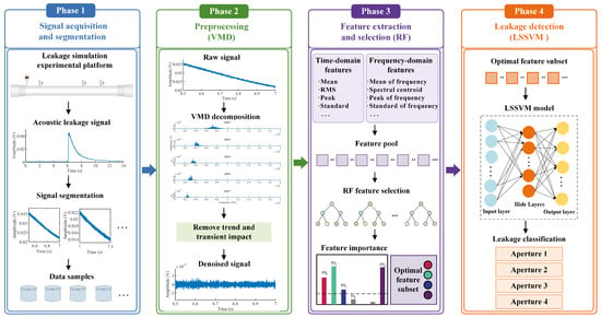
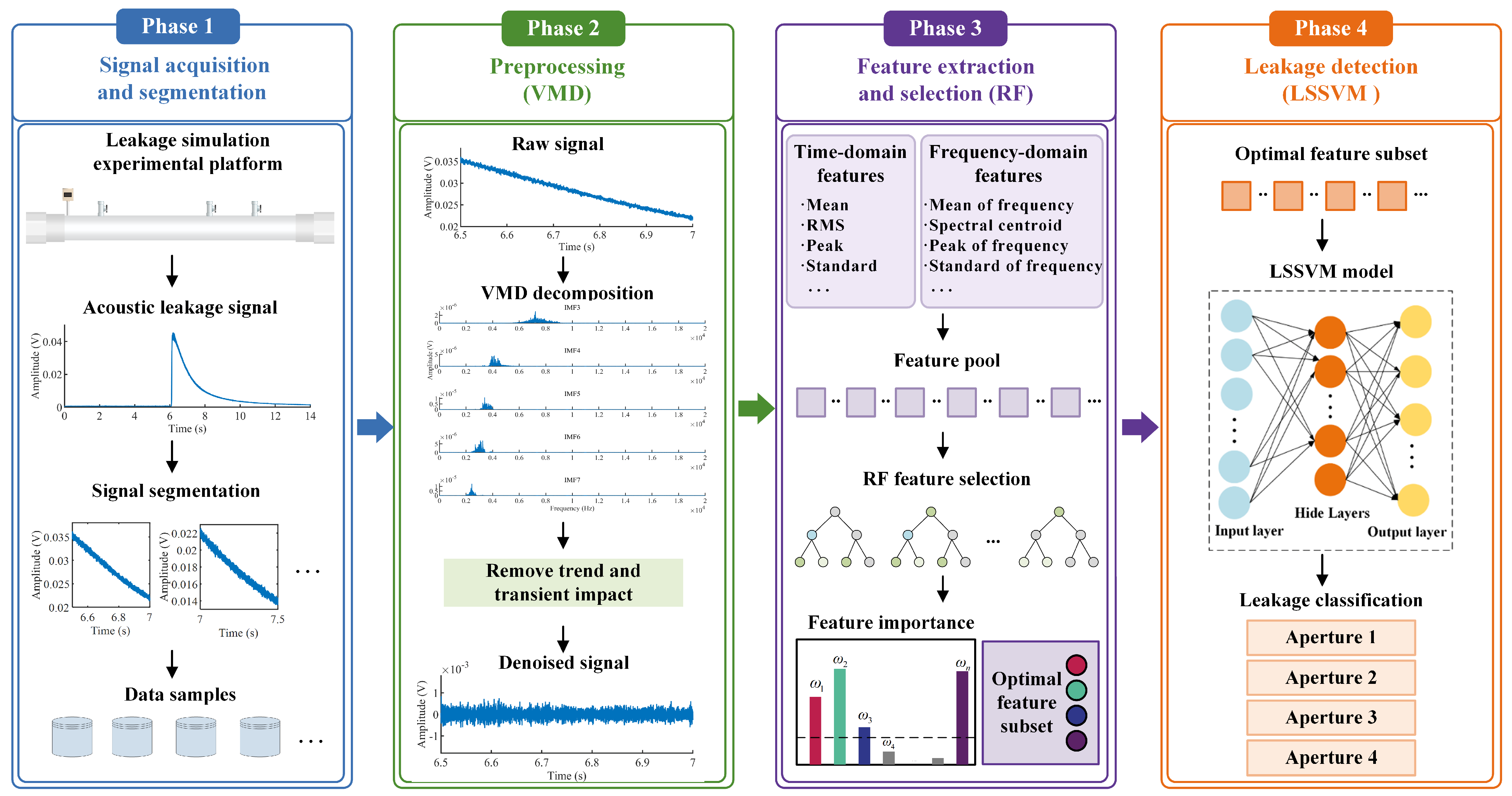
The overall framework of the proposed pipeline unsteady leakage detection method is illustrated in Figure 1, and consists of four phases: signal acquisition and segmentation, preprocessing, feature extraction and selection, and leakage detection.

Figure 1. Overall framework of the proposed pipeline leakage detection method.

In Phase 1, acoustic leakage signals are acquired by the acoustic internal detector and subsequently segmented into multiple signal fragments to generate data samples for subsequent analysis.

In Phase 2, the acquired acoustic signals are preprocessed using the variational mode decomposition (VMD) algorithm. VMD adaptively separates the trend component and transient impacts while suppressing background noise. Since background noise may obscure leakage characteristics, and the trend component together with transient impacts may reduce the generalization capability of the detection method under unsteady leakage conditions, these interference components are effectively suppressed during preprocessing.

In Phase 3, statistical features are extracted from the preprocessed signals in both the time and frequency domains to characterize the leakage state. Random forest (RF) is subsequently employed to evaluate feature importance and select the features that remain relatively stable under unsteady leakage conditions, thereby improving the robustness and accuracy of leakage detection.

Finally, in Phase 4, the selected optimal feature subset is fed into the LSSVM classifier to identify leakage signals corresponding to different leakage apertures.

Compared with conventional leakage detection frameworks, the proposed method is specifically designed for unsteady leakage conditions by integrating VMD-based denoising, RF-based selection of temporally stable features, and LSSVM-based classification to improve the robustness and generalization capability of leakage detection.

3. Basic Theory of Leakage Detection

As illustrated in Figure 1, the proposed pipeline unsteady leakage detection method consists of four sequential phases. These phases are supported by the theoretical foundations presented in this section.

3.1. Aeroacoustic Theory

Aeroacoustic theory primarily addresses the generation and propagation of sound waves in gaseous media, particularly noise issues arising from aerodynamics. In the case of liquid media, the fundamental principles of aeroacoustics remain somewhat applicable, particularly when addressing underwater noise issues [42]. Lighthill’s acoustic analogy theory represents a milestone in aeroacoustics. The central concept of this theory involves forming a non-homogeneous wave equation through mathematical manipulation of the continuity, momentum, and energy conservation equations governing fluid motion, known as Lighthill’s equation [43]:

$${\displaystyle \frac{{\partial }^2{\rho }^{\prime }}{\partial t^2}}-a_0^2{\nabla }^2{\rho }^{\prime }={\displaystyle \frac{{\partial }^2{T}_{ij}}{\partial x_i{x}_j}}$$

(1)

where ρ′ is the density of flow field fluctuations, ρ′ = ρ − ρ₀, ρ is the density under disturbance, ρ₀ is the density without disturbance, kg/m³; a₀ is the sound velocity value under isentropic conditions, m/s; and T_ij is called the Lighthill tensor, Pa.

Ffowcs Williams-Hawkings (FW-H) equation is based on the Lighthill equation, which enables the treatment of sound sources on moving boundaries by incorporating source terms associated with the moving surface [44,45].

$${\displaystyle \frac{{\partial }^2{\rho }^{\prime }}{\partial t^2}}-a_0^2{\nabla }^2{\rho }^{\prime }={\displaystyle \frac{\partial }{\partial t}}\left[{\rho }_0{u}_i{\displaystyle \frac{\partial f}{\partial x_i}}\delta (f)\right]-{\displaystyle \frac{\partial }{\partial x_i}}\left[(p^{\prime }{\delta }_{ij}){\displaystyle \frac{\partial f}{\partial x_i}}\delta (f)\right]+{\displaystyle \frac{{\partial }^2{T}_{ij}}{\partial x_i\partial x_j}}$$

(2)

where u_i represents the component of the incoming flow velocity in the x_i direction, m/s; f denotes the wall function; p′ stands for the far-field sound pressure, Pa; δ_ij is the Kronecker symbol; and δ(f) is the Dirac delta function.

As illustrated in Equation (2), the right side terms of the equation correspond to distinct noise sources. The first term, a monopole source, indicates the rate of change in mass flow, resulting from fluid displacement due to a ruptured pipeline wall. The second term, a dipole source, arises from fluid–structure interactions between the fluid and the pipeline wall, valves, and leakage holes, manifesting as the divergence of pulsating pressure on solid boundaries. The third term, a quadrupole source, represents the turbulent stress of fluid ejected from pipeline leakage holes. The magnitude of these three noise sources is closely linked to the conditions of the pipeline and fluid. Thus, by collecting and analyzing acoustic signals from pipeline leakages, the condition of pipeline leakages can be effectively determined.

3.2. Leakage Acoustic Characteristics

3.2.1. Initial Leakage Stage

When a pipeline leaks, the high-pressure medium inside the pipeline is abruptly released, leading to the formation of shock waves in the gas at the leak point. This causes a sudden change in the particle velocity, pressure, and density of the medium inside the pipeline, subsequently generating leakage sound waves. The sound pressure of these leakage sound waves is described by Equation (3).

$$p=\left\{\begin{array}{c}{p}_0{\mathrm{e}}^{-\left(t-t_1\right)/t_0}, t>t_1\\ 0, t<t_1\hfill \end{array}\right.$$

(3)

where t₁ represents the time when the leakage sound wave is generated, s; t₀ represents the time when the sound pressure decays to ${\mathrm{e}}^{-1}$ times of the original amplitude, s; and p₀ represents the leakage sound pressure at time t₁, Pa.

Performing a Fourier transform on Equation (3), the sound pressure in frequency domain is obtained as Equation (4).

$$p(\omega )=p_0{\displaystyle \frac{1}{\sqrt{{\left(\frac{1}{t_0}\right)}^2+{\omega }^2}}}{\mathrm{e}}^{-\mathrm{j}\omega t_1}$$

(4)

where j is the imaginary unit; $\omega$ is the frequency of sound pressure, Hz.

The corresponding amplitude function is:

$$\left|P(\omega )\right|=p_0{\displaystyle \frac{1}{\sqrt{{\left(\frac{1}{t_0}\right)}^2+{\omega }^2}}}$$

(5)

Different from gas pipelines, liquid pipelines can generate hydrodynamic cavitation during leaks. Consequently, the leakage sound pressure p₀ consists of two components: the maximum water hammer sound pressure p₁, and the cavitation noise sound pressure p₂.

$$p_0=p_1+p_2$$

(6)

where p₁ is the maximum water hammer sound pressure, Pa; p₂ is the cavitation noise sound pressure, Pa.

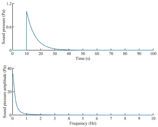
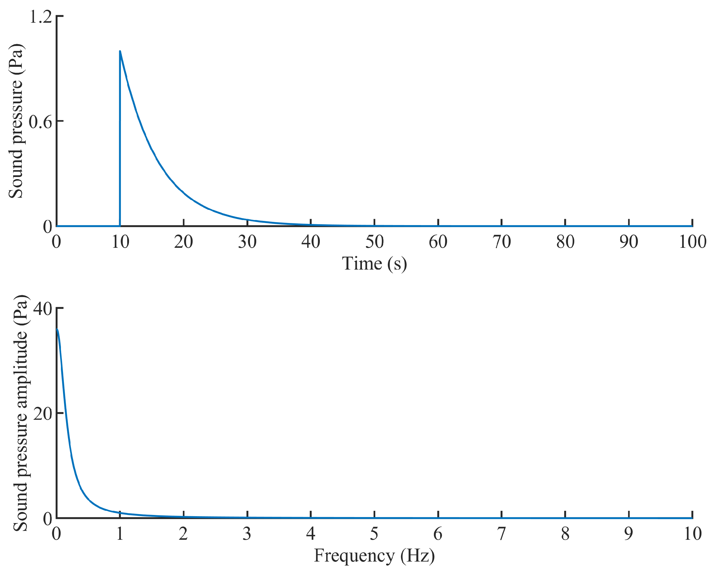
The signal from the pipeline during the initial leakage stage is simulated. Assuming t₀ = 6, t₁ = 10, and p₀ = 1, the time domain waveform and frequency domain amplitude diagram are shown in Figure 2. The time domain signal exhibits a narrow bandwidth near the leakage point, displaying characteristics of a transient shock. The amplitude of the frequency domain signals diminishes as frequency increases, with the energy of the leakage acoustic signals predominantly concentrated in the low-frequency range.

Figure 2. Leakage acoustic signal.

3.2.2. Continuous Leakage Stage

After the leakage, the pipeline enters a stage of continuous leakage. During this stage, the fluid at the leakage point generates turbulence, producing turbulent noise, which can be characterized using a piston-type sound source. The leakage sound pressure [46] can be represented as:

$$p=\mathrm{j}{\omega }_1{\displaystyle \frac{{\rho }_0{u}_0{a}_r^2}{2r}}\left[{\displaystyle \frac{2J_1\left(k{a}_r\sin \theta \right)}{k{a}_r\sin \theta }}\right]{\mathrm{e}}^{\mathrm{j}\left({\omega }_{1}t-kr\right)}$$

(7)

where ${\omega }_1$ is the angular frequency of sound waves, rad/s; ${\rho }_0$ is the medium density, kg/m³; $u_0$ is the sound source vibration amplitude, m; $a_r$ is the sound source radius, m; r is the distance from any test point in the leakage field to the sound source, m; $\theta$ is the angle between the test point and the normal to the sound source cross-section, rad; and $J_1$ is a first-order Bessel function.

3.3. Signal Denoising Based on VMD

VMD, as a form of modal decomposition algorithm, was introduced by Dragomiretskiy and Zosso [47]. The algorithm effectively eliminates the mode mixing problem in EMD, which is widely used for signal processing due to its adaptability and non-recursive characteristics. During the solving process, this algorithm continuously updates the center frequencies of each mode and finally decomposes them into k IMFs. In this paper, k (i.e., the number of IMFs) is set to 7. It should be noted that the number of IMF components is empirically determined based on repeated experiments to achieve a balance between decomposition accuracy and computational complexity. The total sum of all IMFs is equivalent to the original input signal. The expression for the constrained variational problem is shown in Equation (8).

$$\begin{array}{c}\underset{\left\{u_k\right\},\left\{w_k\right\}}{\min }\left\{{\displaystyle \sum _k{‖{\partial }_t\left[\left(\delta (t)+\frac{\mathrm{j}}{\mathsf{\pi }t}\right)\ast u_k(t)\right]{\mathrm{e}}^{\mathrm{j}{w}_{k}t}‖}^2}\right\}\\ \mathrm{s}.\mathrm{t}.{\displaystyle \sum _k}{u}_k=f\end{array}$$

(8)

where x(t) is the original signal; u_k is the kth IMF component; δ(t) is the unit step function; and ω_k is the center frequency corresponding to the kth IMF component.

The previous constrained variational problem is transformed into unconstrained by introducing the Lagrange multiplier λ(t) and the quadratic penalty factor α, as shown in Equation (9).

$$\begin{array}{ll}L(⟨u_k⟩,⟨{\omega }_k⟩,\lambda ):=& \alpha {\displaystyle \sum _k{‖{\partial }_t\left[\left(\partial \left(t\right)+\frac{\mathrm{j}}{\mathsf{\pi }t}\right)\ast u_k\left(t\right)\right]{\mathrm{e}}^{-\mathrm{j}{\omega }_{k}t}‖}_2^2}\\ \hfill +& {‖f(t)-{\displaystyle \sum _k{u}_k}\left(t\right)‖}_2^2+⟨\lambda \left(t\right),f(t)-{\displaystyle \sum _k{u}_k}\left(t\right)⟩\hfill \end{array}$$

(9)

The VMD optimization procedure is as below:

• $\left\{u_k^1\right\}$, $\left\{{\omega }_k^1\right\}$, and ${\widehat{\lambda }}^1$ are initialized, setting n = 0 at this time;
• Incrementing n by 1, ${\widehat{u}}_k$, ${\omega }_k$, and $\widehat{\lambda }$ are updated for all $\omega \ge 0$;

  $${\widehat{u}}_k^{n+1}(\omega )={\displaystyle \frac{\widehat{f}(\omega )-{\displaystyle {\displaystyle \sum _{i=1,i\ne k}^k}{\widehat{u}}_i^{n+1}(\omega )}+{\displaystyle {\displaystyle \sum _{i=1,i\ne k}^k}{\widehat{u}}_i^n(\omega )}+\frac{\widehat{\lambda }(\omega )}{2}}{1+2\alpha {(\omega -{\omega }_k^n)}^2}}$$

  (10)

  $${\omega }_k^{n+1}={\displaystyle \frac{{\displaystyle {\int }_0^{\infty }\omega {\left|{\widehat{u}}_k^{n+1}(\omega )\right|}^2\mathrm{d}\omega }}{{\displaystyle {\int }_0^{\infty }\omega {\left|{\widehat{u}}_k^{n+1}(\omega )\right|}^2\mathrm{d}\omega }}}$$

  (11)

  $${\widehat{\lambda }}^{n+1}(\omega )={\widehat{\lambda }}^n(\omega )+\gamma [\widehat{f}(\omega )-{\displaystyle \sum _{k=1}^k{\widehat{u}}_k^{n+1}(\omega )}]$$

  (12)
• Step (2) is repeated until the constraint condition Equation (13) is satisfied.

  $${\displaystyle \sum _{k=1}^k\frac{{‖{\widehat{u}}_k^{n+1}-{\widehat{u}}_k^n‖}_2^2}{{‖{\widehat{u}}_k^n‖}_2^2}<\epsilon }$$

  (13)

3.4. Time Domain and Frequency Domain Feature Extraction Based on RF

3.4.1. Feature Indexes

In data-based leakage detection methods, feature statistics from the time domain and frequency domain frequently serve as inputs for decision models [48,49], as shown in Table 3 and Table 4.

Table 3. Time domain features of acoustic signals.

Number	Features	Expressions	Number	Features	Expressions
T1	Mean	${\displaystyle \frac{1}{n}}{\displaystyle \sum _{i=1}^n}{x}_i$	T10	Entropy	$-{\displaystyle \sum _{i=1}^n{p}_i}{\log }_2{p}_i$
T2	Root-Mean-Square (RMS)	$\sqrt{{\displaystyle \frac{1}{n}}{\displaystyle \sum _{i=1}^n}{x}_i^2}$	T11	Margin factor	${\displaystyle \frac{Peak}{SRM}}$
T3	Peak	$\max \{\left|\mathit{X}\right|\}$	T12	Crest factor	${\displaystyle \frac{Peak}{RMS}}$
T4	Standard	$\sqrt{{\displaystyle \frac{1}{n}}{\displaystyle \sum _{i=1}^n}{\left[x_i-\mathrm{mean}(\mathit{X})\right]}^2}$	T13	Average rectified value (ARV)	${\displaystyle \frac{1}{n}}{\displaystyle \sum _{i=1}^n\left|x_i\right|}$
T5	Skewness	${\displaystyle \frac{1}{n}}{\displaystyle \sum _{i=1}^n{\left(\frac{x_i-\mathrm{mean}(\mathit{X})}{\mathrm{std}(\mathit{X})}\right)}^3}$	T14	Zero-Crossing rate	${\displaystyle \frac{1}{2}}{\displaystyle \sum _{n=2}^n\left|\mathrm{sgn}(x_i)-\mathrm{sgn}(x_{i-1})\right|}$
T6	Shape factor	${\displaystyle \frac{RMS}{AVR}}$	T15	Peak-to-Peak	$\max \{\mathit{X}\}-\min \{\mathit{X}\}$
T7	Square-Root-Mean (SRM)	${\left({\displaystyle \frac{1}{n}}{\displaystyle \sum _{i=1}^n\sqrt{\left|x_i\right|}}\right)}^2$	T16	Approximate entropy	$\underset{N\to \infty }{\lim }\left[{\Phi }^m(r)-{\Phi }^{m+1}(r)\right]$
T8	Energy	${\displaystyle \sum _{i=1}^n{x}_i^2}$	T17	Impulse factor	${\displaystyle \frac{Peak}{ARV}}$
T9	Kurtosis	${\displaystyle \frac{1}{n}}{\displaystyle \sum _{i=1}^n{\left(\frac{x_i-\mathrm{mean}(\mathit{X})}{\mathrm{std}(\mathit{X})}\right)}^4}$

Note: X is the time domain signal; $\mathrm{sgn}(\cdot )$ is the sign function; p_i is the proportion of the energy of a point in the signal to the total energy, $p_i=x_i^2/{\displaystyle \sum _{i=1}^n}{x}_i^2$; ${\Phi }^m(r)$ represents the similarity of the vector sets at two different time points.

Table 4. Frequency domain features of acoustic signals.

Number	Features	Expressions	Number	Features	Expressions
F1	Mean of frequency	${\displaystyle \frac{1}{n}}{\displaystyle \sum _{i=1}^n{y}_i}$	F5	Peak frequency	${\mathit{f}}_i{|}_{y_i=\max \{\mathit{Y}\}}$
F2	Spectral centroid	${\displaystyle \frac{\mathit{Y}\times {\mathit{f}}^T}{{\displaystyle \sum _{i=1}^n{y}_i^2}}}$	F6	Energy of frequency	${\displaystyle \sum _{i=1}^n{y}_i^2}$
F3	Peak of frequency	$\max \{\mathit{Y}\}$	F7	Root-Mean-Square of frequency	$\sqrt{{\displaystyle \frac{1}{n}}{\displaystyle \sum _{i=1}^n{y}_i^2}}$
F4	Standard of frequency	$\sqrt{{\displaystyle \frac{1}{n}}{\displaystyle \sum _{i=1}^n{\left[y_i-\mathrm{mean}(\mathit{Y})\right]}^2}}$

Note: Y is the amplitude spectrum of X after Fourier transform; f is the corresponding frequency.

3.4.2. Feature Selection Based on RF

RF is used as a feature selection method for acoustic signal in this section. The advantages of RF are primarily its robust predictive capability and unbiasedness towards data, with significant applications in feature selection [50,51].

When constructing a decision tree using the RF algorithm, a set of data is obtained through random sampling for training the decision tree, and the data not sampled becomes Out of Bag (OOB). OOB is utilized for evaluating the decision tree’s performance. In application, the minimum OOB error rate is selected to assess the significance of each feature. The fundamental concept is to introduce noise to a feature, which decreases prediction accuracy. The extent of this accuracy drop indirectly indicates the feature’s importance, serving as a basis for ranking feature significance. The detailed process of feature selection is as follows.

• The mean prediction error of decision tree i is calculated using the OOB data, as described in Equation (14).

  $$E{1}_i={\displaystyle \frac{1}{n}}{\displaystyle \sum _{k=1}^n(y_k-{\widehat{y}}_k)}$$

  (14)

  where n is the number of OOB data points, $\widehat{y}$ is the model’s predicted label, and y is the true label.
• With the other features remaining constant, the noise disturbance is introduced to feature j and the mean prediction error of decision tree i is recalculated, as described in Equation (15).

  $$E{2}_{ij}={\displaystyle \frac{1}{n}}{\displaystyle \sum _{k=1}^n(y_k-{\widehat{y}}_k)}$$

  (15)
• Assuming an RF comprises N decision trees, the importance of feature j is determined as follows.

  $$I_j={\displaystyle \frac{1}{N}}{\displaystyle \sum _{i=1}^N(E{2}_{ij}-E{1}_i)}$$

  (16)
• The above steps are repeated for all remaining features until all have been exhausted. Subsequently, sorting is performed to establish the importance ranking of each feature.

In practical applications, the ranking of feature importance guides the selection of the optimal feature subset. In this study, the number of decision trees in the RF model is set to 10 based on preliminary experiments to achieve a balance between feature selection stability and computational efficiency.

3.5. Pipeline Leakage Detection Based on LSSVM

The LSSVM algorithm, a variant of the SVM algorithm, converts the convex quadratic programming problem into a linear optimization problem. It not only ensures computational accuracy but also simplifies the training process and enhances solving speed [52]. This paper uses the LSSVM algorithm for the pipeline leakage apertures classification.

The fundamental concept of the LSSVM algorithm involves utilizing nonlinear functions to map the input space into a high-dimensional feature space, subsequently identifying a suitable hyperplane within this space to facilitate data classification. Assuming the sample set $Q=\{x_i,y_i\}(i=1,2,3,\dots ,n)$, the sample size is n, where the input quantity is x_i and the output quantity is y_i. By mapping the sample set Q to the high-dimensional feature space F, the classification function is expressed as below.

$$f(x)=\mathrm{sgn}({\mathit{\omega }}^{\mathrm{T}}\mathit{\phi }(x)+b)$$

(17)

where $\mathit{\omega }$ is the weight factor, b is the bias factor, and $\mathit{\phi }(\cdot )$ represents the nonlinear mapping.

The optimization objective and constraint objective of the LSSVM algorithm are:

$$\left\{\begin{array}{c}\min J(\omega ,e)={\displaystyle \frac{\parallel \mathit{\omega }{\parallel }^2}{2}}+{\displaystyle \frac{1}{2}}c{\displaystyle \sum _{i=1}^n{e}_i^2}\\ \mathrm{s}.\mathrm{t}. y_i[{\mathit{\omega }}^{\mathrm{T}}\mathit{\phi }(x_i)+b]=1-e_i (i=1,2,3,\dots ,n)\end{array}\right.$$

(18)

where J is the loss function; c is the penalty coefficient; e_i is the error term.

On the basis of Equation (18), the Lagrange equation is constructed as below.

$$L(\omega ,b,e,\alpha )=J(\omega ,e)-{\displaystyle \sum _{i=1}^n{\alpha }_i[y_i({\omega }^{\mathrm{T}}f(x)+b)-1+e_i]}$$

(19)

where ${\alpha }_i$ is the Lagrangian operator.

By combining Equations (18) and (19), a system of linear equations can be obtained as below.

$$\left[\begin{array}{cc}0\hfill & -{\mathit{Y}}^{\mathrm{T}}\\ \mathit{Y}\hfill & {\mathit{\Omega }}_{i,j}+{\mathit{C}}^{-1}\mathit{I}\end{array}\right]\left[\begin{array}{c}b\\ \alpha \end{array}\right]=\left[\begin{array}{c}0\\ {\mathit{I}}_n\end{array}\right]$$

(20)

where $\mathit{\Omega }=y_i{y}_j{\mathit{\phi }}^{\mathrm{T}}(x_i)\mathit{\phi }(x_i)=y_i{y}_j\mathit{K}(x_i,x_j)$, $\mathit{K}(x_i,x_j)$ is the kernel function, $j=1,2,\dots ,n$; ${\mathit{y}}^{\mathrm{T}}=[y_1,y_2,\dots ,y_n]$; I is the identity matrix; ${\mathit{I}}_n={\left[1,\dots ,1\right]}^{\mathrm{T}}$.

Finally, the values of α and b can be estimated using the method of least squares. The derived decision function is as below.

$$f(x)=\mathrm{sgn}\left[{\displaystyle \sum _{i=1}^n{\alpha }_i{y}_{i}K(x,x_i)+b}\right]$$

(21)

In practical applications, by inputting test samples into a trained decision classification model based on the LSSVM model, the corresponding leakage aperture can be determined, thereby achieving effective pipeline leakage detection. In this paper, to achieve effective detection of unsteady leakage, the two parameters of the LSSVM model (i.e., penalty coefficient c and kernel function bandwidth parameter ${\sigma }^2$) are set to 16 and 0.05, respectively.

4. Simulation Experiment of the Unsteady Micro-Leakage

This section describes the experimental design for pipeline unsteady micro-leakage simulation, including the experimental objectives, setup, and data acquisition procedure. These experiments provide the acoustic signal dataset used to validate the proposed leakage detection method.

4.1. Experimental Objective

Pipeline leakage is typically accompanied by complex acoustic emission phenomena arising from the interactions among the leaking fluid, the pipeline structure, and the surrounding medium. The primary objective of this experiment is to investigate the acoustic characteristics of pipeline unsteady leakage under controlled and repeatable conditions and to acquire representative acoustic signals for validating the proposed leakage detection method. The position of the hydrophone represents the position of the acoustic inner detector. The experiment uses the method of continuous leakage after pressurization to simulate the unsteady leakage. The internal pressure of the pipeline will continue to decrease as the leakage occurs. Acoustic internal inspection signals generated by leakage under different initial operating pressures and leakage apertures are collected, providing a reliable dataset for the training and testing of the leakage detection method.

4.2. Experimental Scheme

Experimental research was conducted using the acoustic internal inspection method, distinct from traditional leakage acoustic external detection methods. The hydrophone was positioned inside the pipeline, and the leakage acoustic signal was able to propagate through the fluid medium to the sensor vicinity [53].

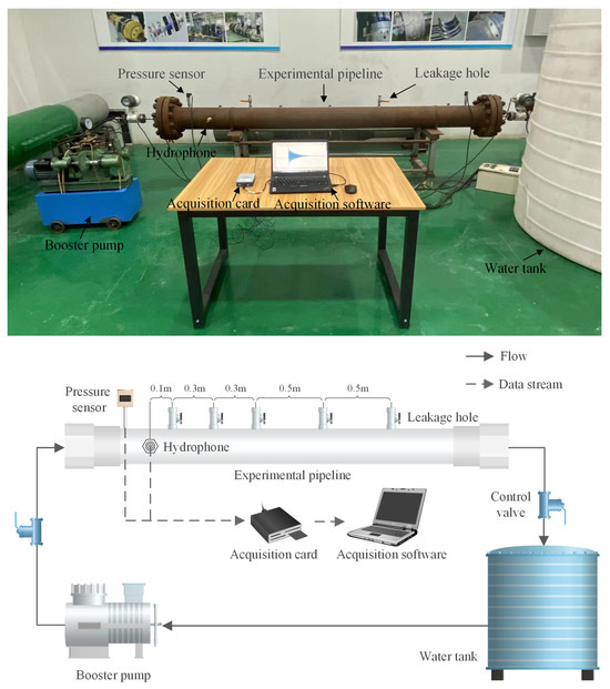
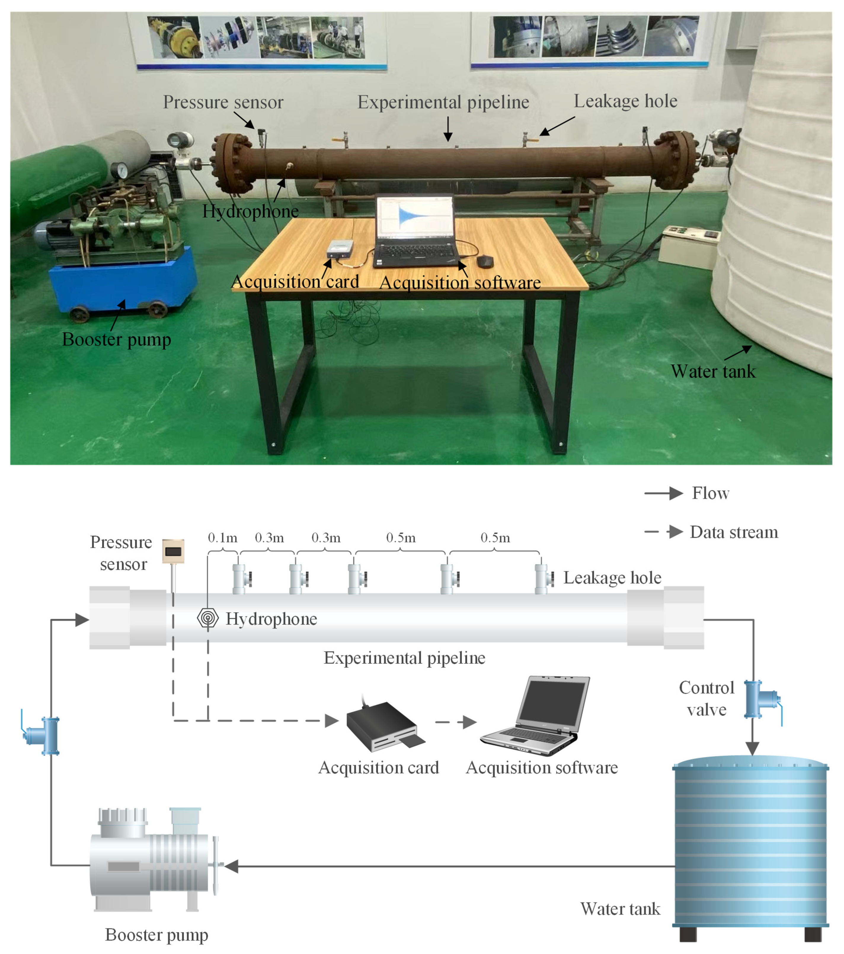
The experimental platform comprised pipeline, pressurization device, water tanks, pressure sensors, hydrophones, and acquisition system, as shown in Figure 3. The pipeline was made of DN219mm steel pipe, with a wall thickness of 6 mm and a length of 2.5 m. Water was used as the medium of pipeline transportation. The hydrophone was set at 400 mm from the left end of the pipeline. Pressure sensors were set at both ends of the pipeline. Four kinds of bolts with different opening diameters of 0.6, 0.8, 1.0 and 2.0 mm were used in the experiment. The simulated pressure range for the experiment was set between 0.2 and 1.6 MPa. Since the frequency spectrum of pipeline leakage signals was in a wide range, the selection of an acoustic sensor with both a broad frequency capacity and high sensitivity was imperative. The TC4013 hydrophone from RESON, a Danish company, was chosen for the experimental setup. The sensor features a linear frequency range of 1–50 kHz, an overall frequency response of 1 Hz–170 kHz, and a receiving sensitivity of −217 dB, which together fully meet the experimental requirements. Additionally, a high-speed real-time data acquisition system was established, employing an NI collector and LabVIEW 2021 software.

Figure 3. Leakage simulation experimental platform.

The acquisition system sampling frequency was set at 40 kHz, gathering acoustic data on pipeline leakage at various leakage locations (0.1, 0.4, 1.2, and 1.7 m from the leakage source), with different aperture sizes (0.6, 0.8, 1.0, and 2.0 mm), and under varying operational pressures (0.6, 1.2, and 1.6 MPa). Initially, the experiment followed the scheme by selecting the specified bolt and installing it at the chosen leakage point. Subsequently, the pipeline was pressurized to the designated level. Finally, the valve of the perforated bolt was opened for testing and data collecting.

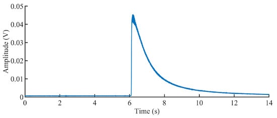
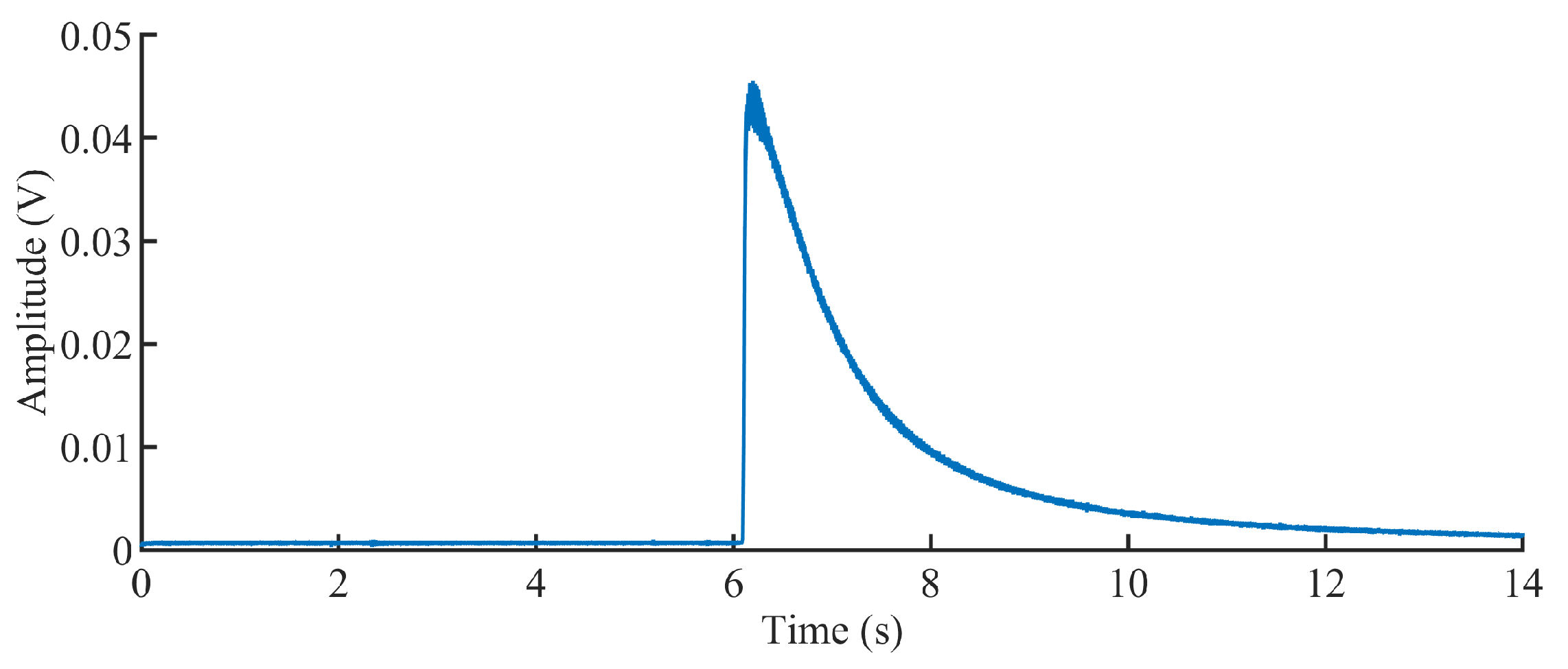
As a representative example, the acoustic signal obtained under an operating pressure of 1.2 MPa, a leakage aperture of 2.0 mm, and a leakage location of 1.2 m is presented in Figure 4. The pipeline leaked at 6.3 s, and the acoustic signal displayed significant impact characteristics in the time domain, followed by a gradual decrease in amplitude. The entire leakage process was accompanied by a significant pressure drop, which affects the leakage rate. Therefore, the entire leakage process demonstrated unsteady leakage characteristics. The acquired acoustic signals under different operating conditions constitute the experimental dataset used for subsequent leakage detection. The effectiveness of the proposed detection method is evaluated based on these data in the following section.

Figure 4. Time domain waveform of leakage acoustic signal.

5. Pipeline Leakage Detection Results and Analysis

This section presents the experimental results and corresponding analysis of the proposed pipeline unsteady leakage detection method.

5.1. Noise Reduction of Leakage Acoustic Signal

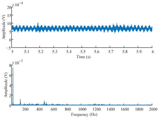
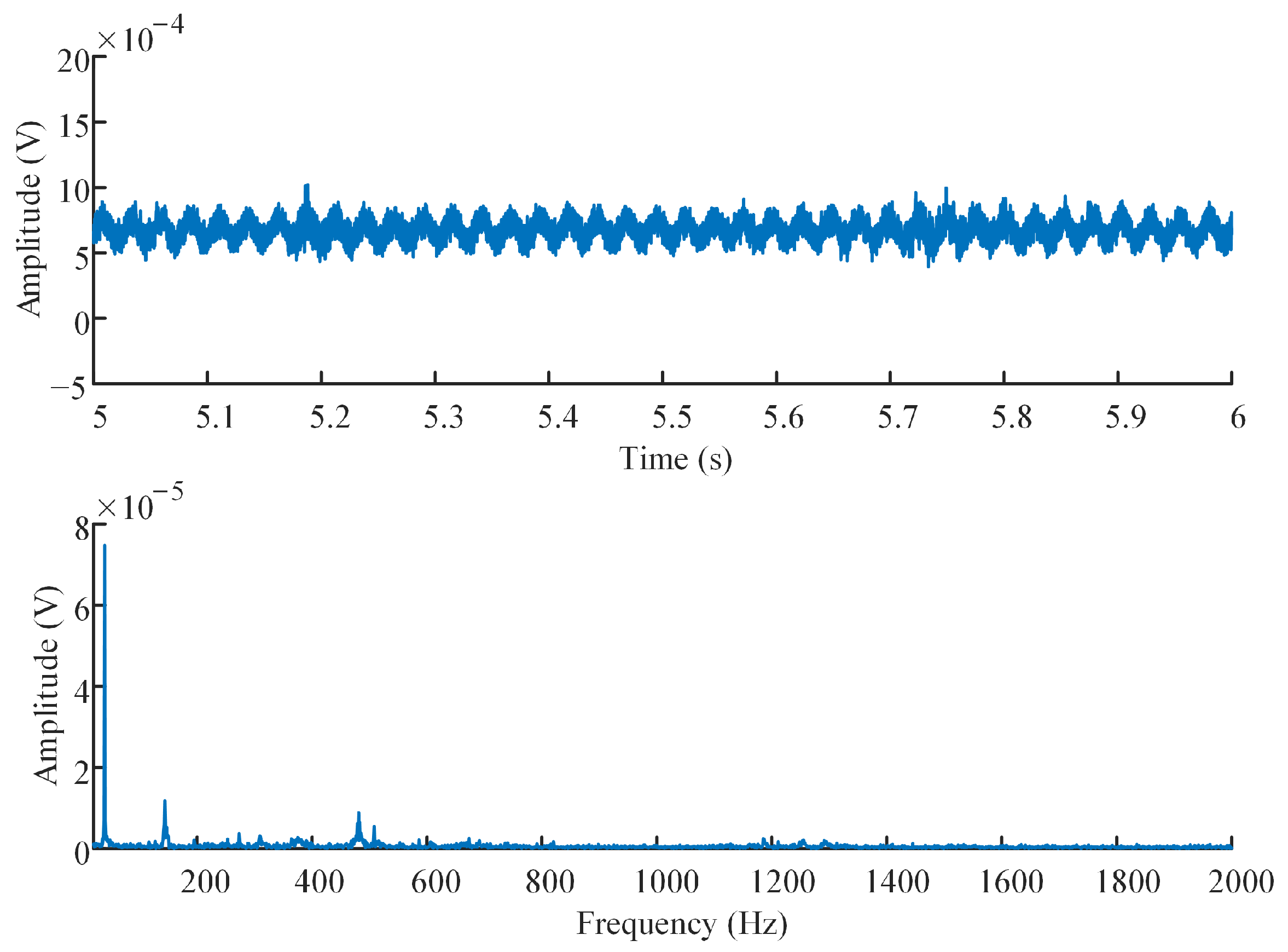
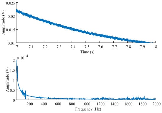
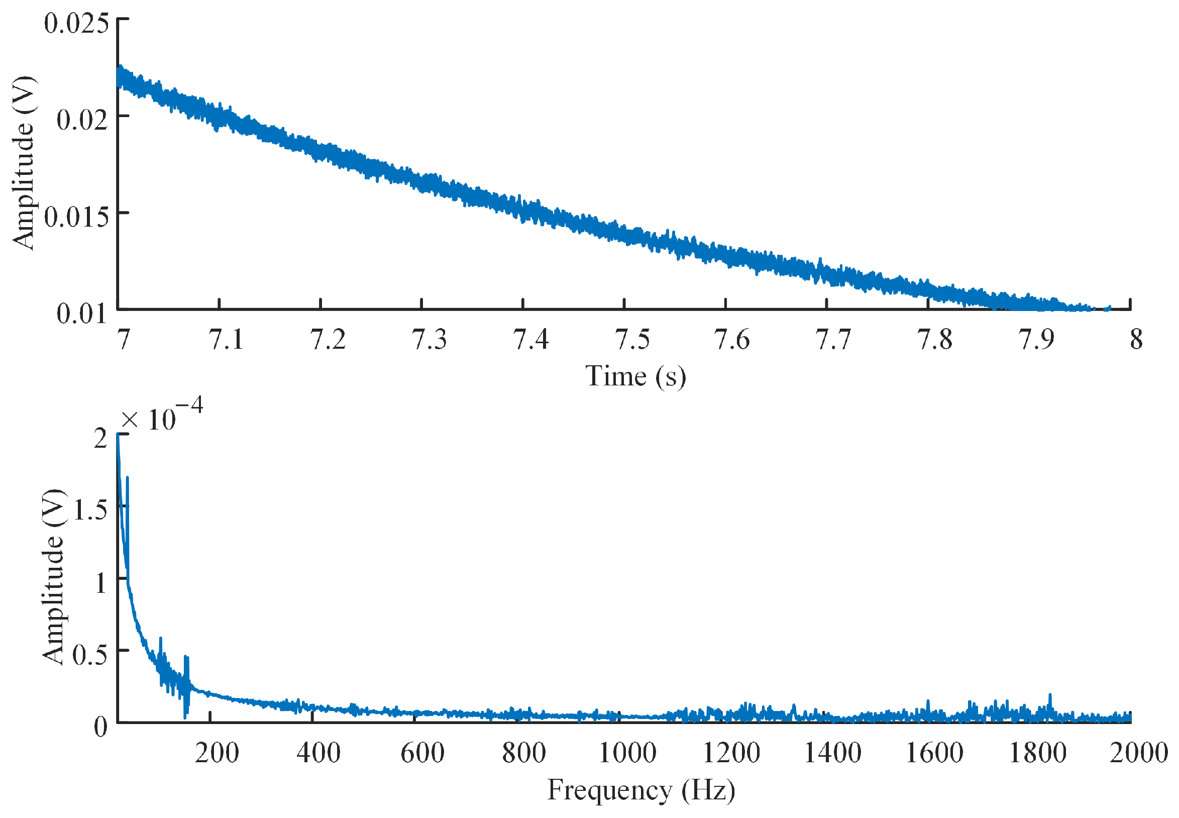
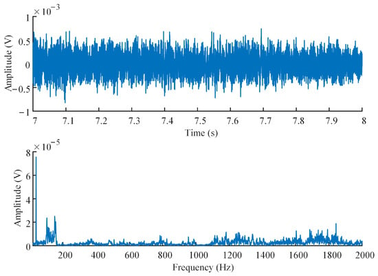
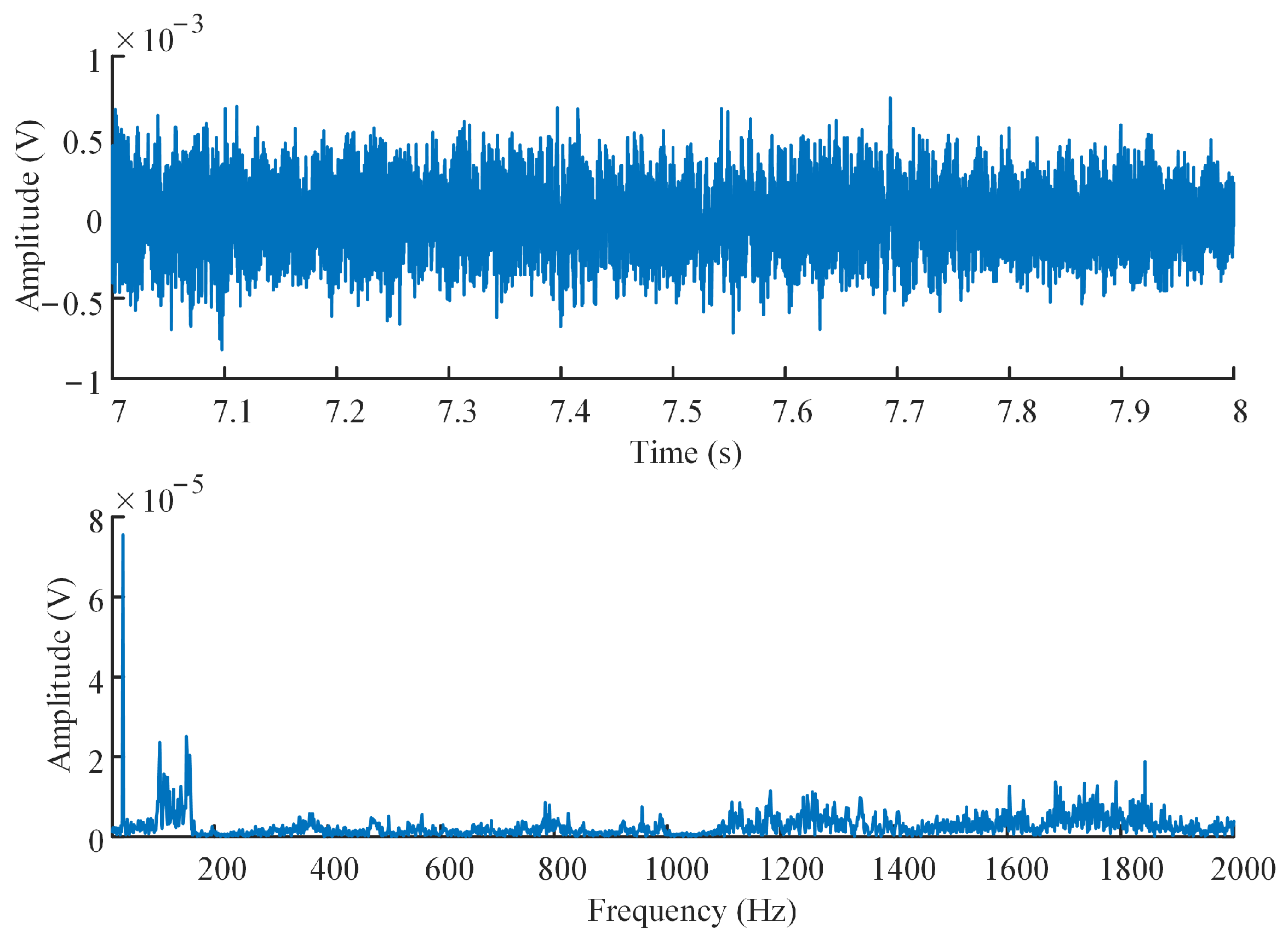
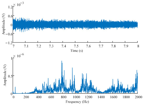
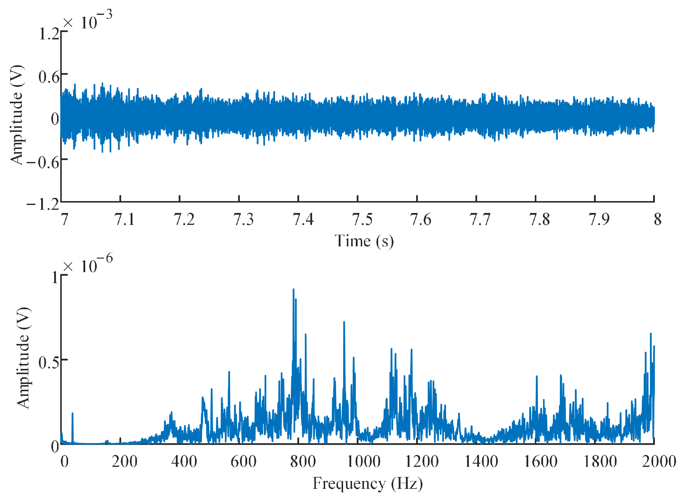
To illustrate the signal denoising process, the acoustic signal acquired under a representative operating condition (operating pressure of 1.2 MPa, leakage aperture of 2.0 mm, and leakage location of 1.2 m) is used as an example. The corresponding time domain waveforms and frequency spectra before and after leakage are shown in Figure 5 and Figure 6, respectively. The ordinate represents the acoustic signal amplitude (V). Before leakage, the time domain signal remains relatively stable with random fluctuations. After leakage occurs, the signal amplitude gradually decreases as the internal pipeline pressure continuously decays. In the frequency domain, the spectral energy is primarily concentrated in the low-frequency range.

Figure 5. Acoustic signal before leakage.

Figure 6. Acoustic signal after leakage.

Before feature extraction, the trend component is removed to eliminate the slowly varying pressure-decay trend, thereby ensuring that the extracted features primarily reflect leakage-related characteristics rather than pressure-dependent variations. Polynomial detrending is a widely adopted preprocessing technique for eliminating low-frequency baseline variations in nonstationary signals [54]. In this study, a cubic polynomial was employed because it provides sufficient flexibility to accurately model the slowly varying nonlinear trend caused by the gradual pressure decay, while avoiding unnecessary fitting complexity. The detrending result is shown in Figure 7.

Figure 7. Leakage acoustic signal after removing trend component.

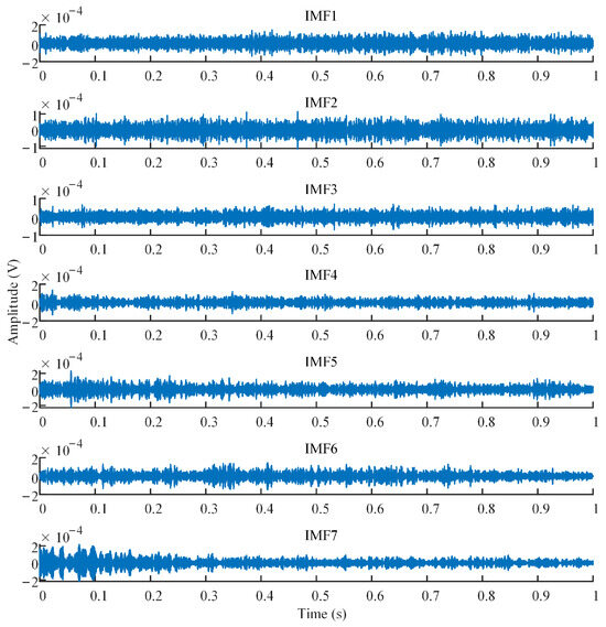
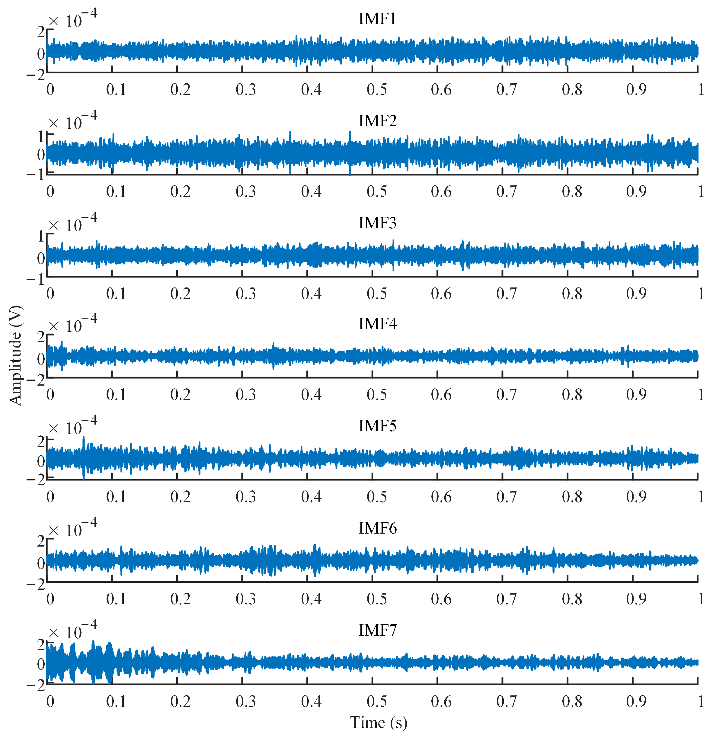
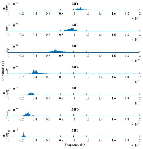
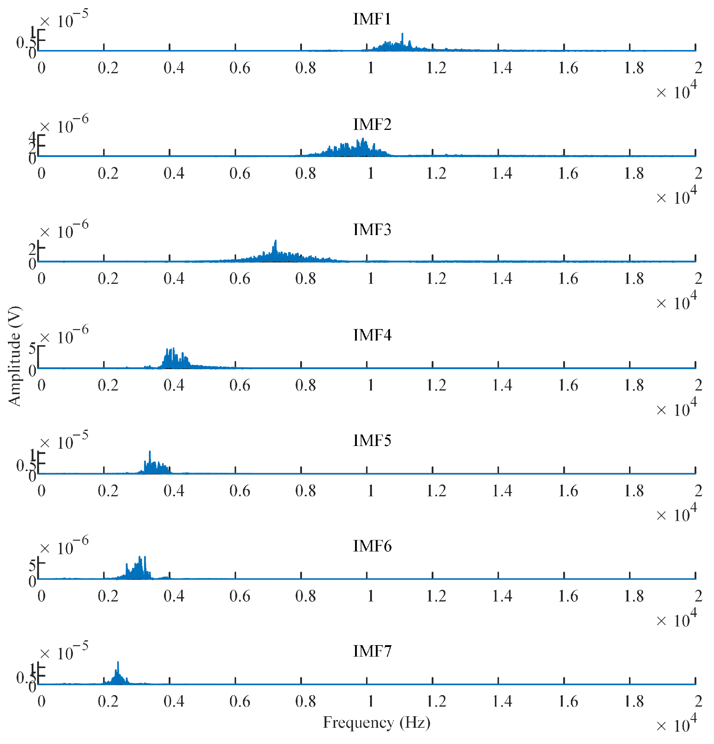
The leakage acoustic signal is decomposed by using the VMD algorithm, obtaining 7 IMF components and a residual component. The time domain and frequency domain for each IMF component are shown in Figure 8 and Figure 9. The leakage acoustic signal is decomposed into multiple intrinsic mode functions with distinct frequency characteristics. No obvious mode aliasing or over-decomposition is observed, indicating that the selected VMD parameters are appropriate for the analyzed signal.

Figure 8. Time domain waveforms of IMF components.

Figure 9. Frequency domain waveforms of IMF components.

The selection of IMF components is based on the correlation coefficients between each IMF component and the original signal. In this paper, the IMF components are selected based on the criterion $K\ge \max (K)/2$. According to Table 5, IMF1-IMF2 and IMF4-IMF7 are chosen as the effective components.

Table 5. Correlation coefficients between various IMF components and x(t).

	IMF1	IMF2	IMF3	IMF4	IMF5	IMF6	IMF7
Correlation coefficient K	0.2779	0.2366	0.1592	0.2640	0.3739	0.3731	0.3805

The signal is reconstructed by selecting the effective components. The time domain and frequency domain waveforms of the reconstructed leakage acoustic signal are illustrated in Figure 10. After VMD denoising, the trend component is removed from the time domain signal, enhancing the features of the frequency domain signal.

Figure 10. Leakage acoustic signal after reconstruction.

5.2. Feature Extraction of Leakage Acoustic Signal

The time domain (T1–T17) and frequency domain (F1–F7) features were extracted from the reconstructed signal x_r(t) shown in Figure 10, resulting in a 24-dimensional feature vector for the leakage acoustic signal. However, the high dimensionality of these features results in considerable redundancy. For unsteady leakage, the selected features must remain relatively constant over time under these conditions. Consequently, the RF algorithm is employed to filter the conventional time and frequency domain features. The filtered features must effectively indicate the pipeline’s leakage aperture.

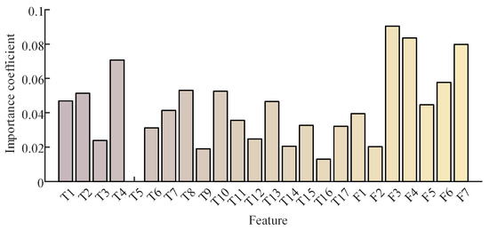
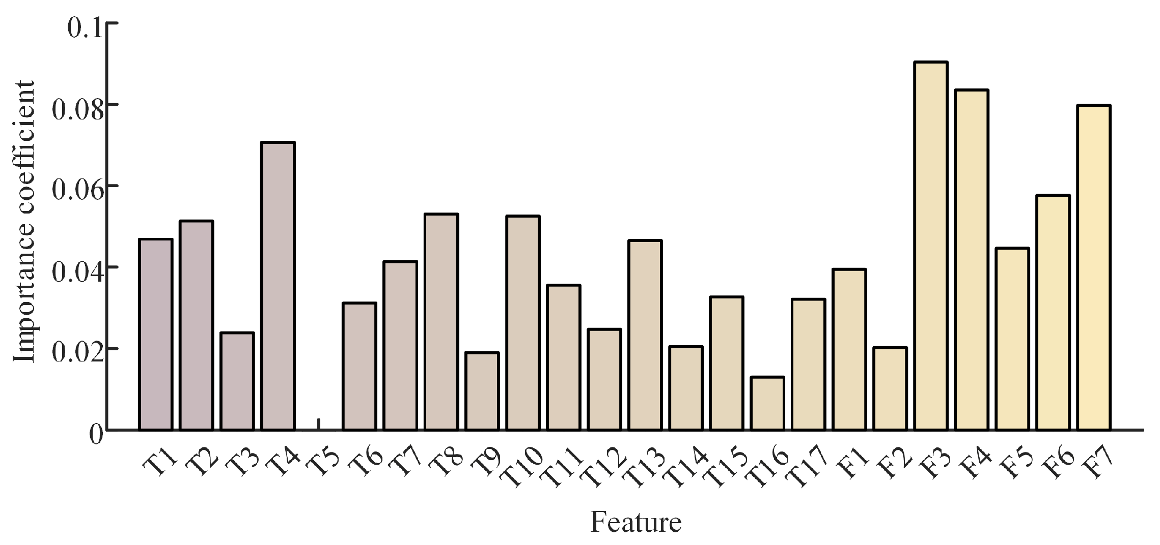
The random forest model is set to include 10 decision trees; the importance coefficient I of each feature is calculated, and their significance is ranked. The importance of each feature is illustrated in Figure 11. Additionally, the optimal feature subset is constructed according to the specific criterion $I\ge \max (I)/2$, retaining the highly important features, as shown in Table 6.

Figure 11. Importance coefficient of each feature.

Table 6. Optimal feature subset.

Number	Feature	Importance Coefficient	Number	Feature	Importance Coefficient
1	F3	0.0904	6	T8	0.0530
2	F4	0.0836	7	T10	0.0526
3	F7	0.0797	8	T2	0.0513
4	T4	0.0707	9	T1	0.0469
5	F6	0.0577	10	T13	0.0466

5.3. Classification Detection of Leakage Acoustic Signal

The pipeline leakage acoustic signals with four aperture sizes of 0.6 mm, 0.8 mm, 1.0 mm, and 2.0 mm are selected under the same initial leakage pressure (1.6 MPa) as the experimental data, with the hydrophone positioned 0.1 m from the leakage. The signals are segmented using 2000 data points with no overlap between samples. The feature extraction is performed according to Table 6. For each leakage aperture size, 80 samples are collected, resulting in a total of 320 samples. The dataset of unsteady leakage acoustic signals is presented in Table 7.

Table 7. Unsteady leakage acoustic signal dataset.

Label	Leakage Aperture	Quantity
1	0.6 mm	80
2	0.8 mm	80
3	1.0 mm	80
4	2.0 mm	80

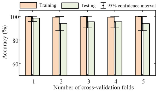
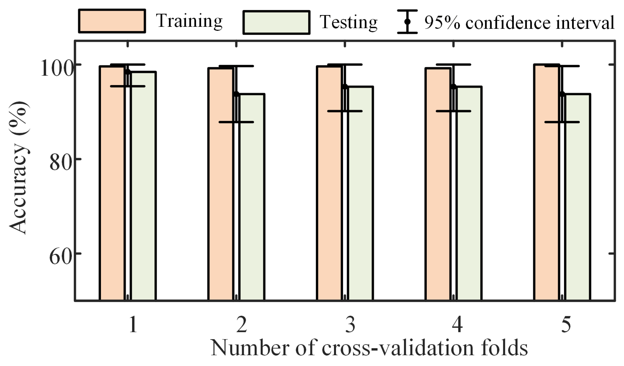
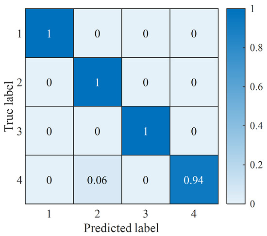
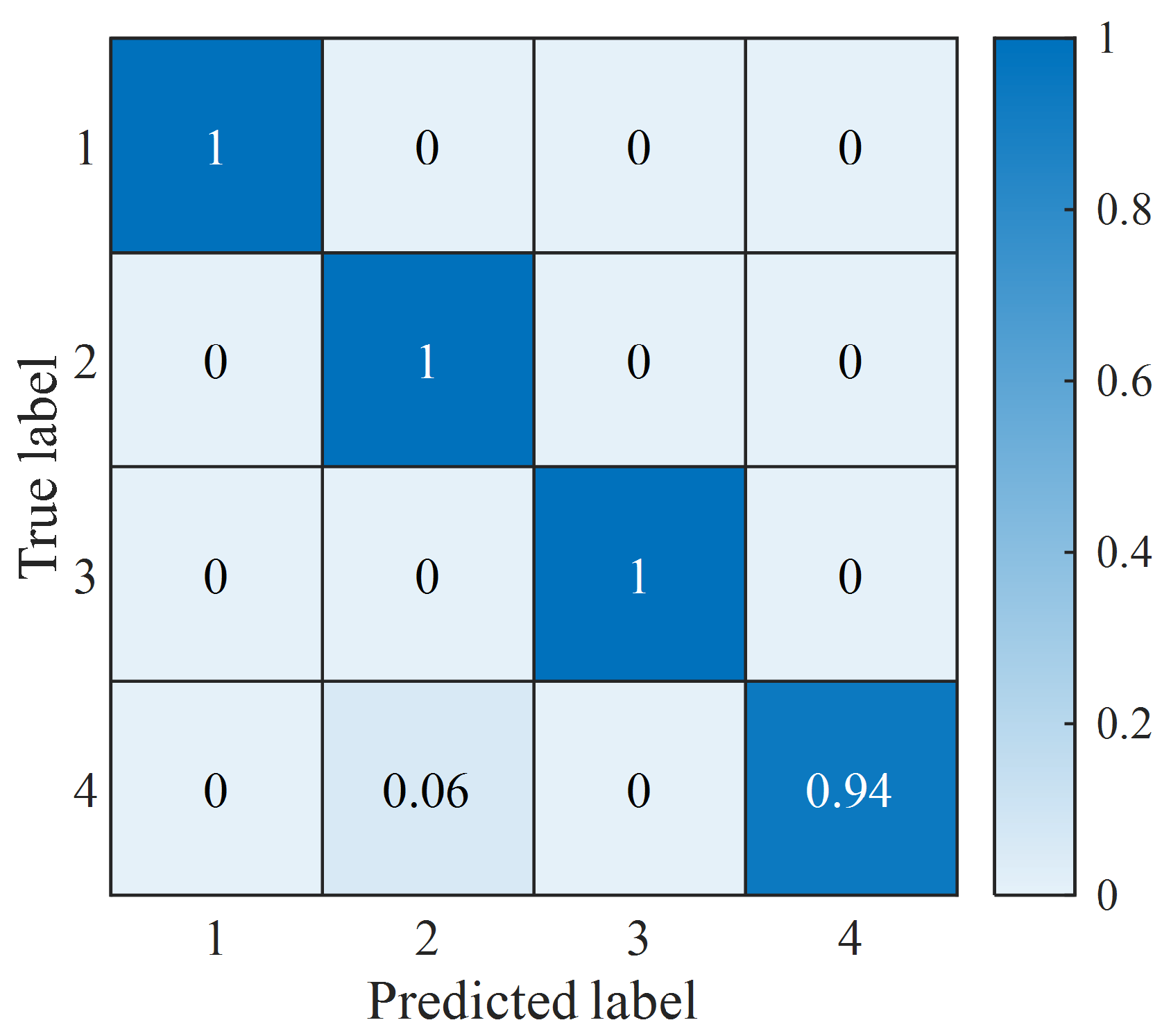
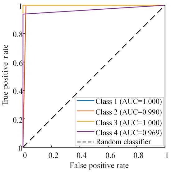
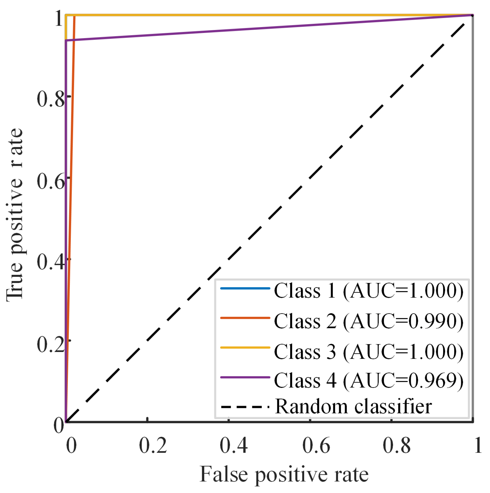
Before being input into the model, all features are normalized. A 5-fold cross-validation strategy is adopted to evaluate the generalization performance of the proposed model [55], where the dataset is randomly divided into five subsets, with four subsets used for training and the remaining subset used for testing in each iteration. The cross-validation results are shown in Figure 12. The average detection accuracy of the training set and the test set is 99.38% and 95.31%, respectively. The 95% confidence interval of the average accuracy of the test set is [93.00%, 97.63%]. The confusion matrix and the receiver operating characteristic (ROC) curve corresponding to the best-performing test fold are shown in Figure 13 and Figure 14. The results show that the pipeline leakage detection model based on LSSVM can realize the effective detection of leakage aperture.

Figure 12. Results of cross-validation.

Figure 13. Confusion matrix.

Figure 14. ROC curve.

5.4. Analysis of Detection Results

The detection performance was evaluated using Accuracy, Precision, Recall, F1-score, and Kappa coefficient, which are widely adopted performance metrics for classification models [56,57,58].

$$Accuracy={\displaystyle \frac{TP+TN}{TP+TN+FP+FN}}$$

(22)

$$Precision={\displaystyle \frac{TP}{TP+FP}}$$

(23)

$$Recall={\displaystyle \frac{TP}{TP+FN}}$$

(24)

$$F1=2\times {\displaystyle \frac{Precision\times Recall}{Precision+Recall}}$$

(25)

$$\kappa ={\displaystyle \frac{P_{\mathrm{o}}-P_{\mathrm{e}}}{1–P_{\mathrm{e}}}}$$

(26)

where TP is the number of True Positives, FP is the number of False Positives, FN is the number of False Negatives, TN is the number of True Negatives, P_o is the observed consistency rate, and P_e is the random consistency rate.

To verify the rationality of the proposed method, ablation experiments were carried out. The baseline models include: LSSVM (c = 10, ${\sigma }^2$ = 120), RF-LSSVM (c = 10, ${\sigma }^2$ = 4) and VMD-LSSVM (c = 20, ${\sigma }^2$ = 12). The remaining parameters of the basic models are consistent with the VMD-RF-LSSVM model.

The results of ablation experiments are shown in Table 8. The LSSVM model directly uses these 24 extracted features as input. However, due to the existence of redundant features and noise, its detection performance is relatively limited. By introducing the RF-based feature selection method, the performance of the RF-LSSVM model is improved. This shows that the removal of redundant features can enhance the discriminant ability of LSSVM classifier. The VMD-LSSVM model performs signal denoising before feature extraction, which significantly improves the classification accuracy and robustness. This shows that improving the signal quality in the preprocessing stage plays a vital role in enhancing model performance. Overall, ablation experimental results show that both feature selection and signal denoising have a positive impact on the proposed framework. The ablation experiments demonstrate the effectiveness of the proposed method.

Table 8. Comparative performance of ablation experiments.

	Training					Testing
Models	Accuracy	Precision	Recall	F1	Kappa	Accuracy	Precision	Recall	F1	Kappa
LSSVM	0.9242	0.9348	0.9242	0.9241	0.8990	0.8906	0.9067	0.8906	0.8887	0.8542
VMD-LSSVM	0.9680	0.9693	0.9680	0.9679	0.9573	0.9094	0.9159	0.9094	0.9091	0.8792
RF-LSSVM	0.9539	0.9565	0.9539	0.9536	0.9385	0.9344	0.9391	0.9344	0.9337	0.9125
VMD-RF-LSSVM	0.9938	0.9939	0.9938	0.9937	0.9917	0.9531	0.9578	0.9531	0.9529	0.9375

To further evaluate the effectiveness of the proposed pipeline unsteady leakage detection method, comparative experiments were conducted with several representative machine learning (ML) and deep learning (DL) methods. The compared ML methods include XGBoost (NumBoost = 10, MaxDepth = 4), AdaBoost (NumBoost = 10, MaxNumSplits = 4), CatBoost (NumBoost = 10, MaxDepth = 4), and KNN (NumNeighbors = 5). The compared DL methods include CNN, BiLSTM, and ResNet-50. The network architectures and hyperparameters of the DL methods were configured according to Zhao et al. [59]. For the ML methods, the 24 manually extracted time and frequency domain features were used as inputs, whereas the DL methods directly used the raw time-series signals as inputs.

The quantitative comparison results are summarized in Table 9. Ensemble learning-based methods (XGBoost, AdaBoost, and CatBoost) generally outperform KNN, indicating that ensemble learning strategies are more effective in capturing complex feature relationships in leakage signals. Although XGBoost and CatBoost achieve relatively high test accuracies, their performances remain inferior to that of the proposed VMD-RF-LSSVM method. In contrast, the DL methods exhibit limited detection capability, with test accuracies below 55%. This limitation is mainly attributed to the nonstationary characteristics of the leakage signals, noise interference, limited sample size, and the lack of sufficient prior information. Benefiting from VMD-based signal denoising, RF-based feature selection, and LSSVM-based classification, the proposed VMD-RF-LSSVM method achieves the best overall performance, with a test accuracy of 95.31%, an F1 score of 0.9529, and a Kappa coefficient of 0.9375. These results demonstrate that the proposed method provides a more reliable and effective solution for pipeline unsteady leakage detection than conventional ML and DL methods.

Table 9. Comparative performance of different models.

	Training					Testing
Models	Accuracy	Precision	Recall	F1	Kappa	Accuracy	Precision	Recall	F1	Kappa
XGBoost	0.9836	0.9839	0.9836	0.9836	0.9781	0.9344	0.9382	0.9344	0.9333	0.9125
AdaBoost	0.9539	0.9586	0.9539	0.9540	0.9385	0.9156	0.9247	0.9156	0.9135	0.8875
CatBoost	0.9742	0.9747	0.9742	0.9741	0.9656	0.9344	0.9387	0.9344	0.9341	0.9125
KNN	0.8477	0.8534	0.8477	0.8448	0.7969	0.7656	0.7803	0.7656	0.7550	0.6875
CNN	0.5391	0.5599	0.5391	0.4712	0.3854	0.5156	0.5118	0.5156	0.4606	0.3542
BiLSTM	0.5625	0.5912	0.5625	0.5370	0.4167	0.4594	0.4214	0.4594	0.4101	0.2792
Resnet50	0.5438	0.6123	0.5437	0.4796	0.3917	0.5344	0.6153	0.5344	0.4645	0.3792
VMD-RF-LSSVM	0.9938	0.9939	0.9938	0.9937	0.9917	0.9531	0.9578	0.9531	0.9529	0.9375

5.5. Comparisons with Relevant Research Works

In the existing research, most methods are mainly based on two ideas: one is the combination of handcrafted features and traditional ML classifiers, and the other is the DL-based method that directly processes original signals. Feature-based methods, such as using SVM, RF, or ensemble learning algorithms, often face the challenge of performance degradation when dealing with unsteady signals. DL-based methods require large-scale labeled datasets [36]. In contrast, the proposed VMD-RF-LSSVM model unifies signal decomposition, feature selection and classification. This model demonstrates excellent detection performance in small-sample, unsteady leakage detection. From the comparison results, the proposed method is superior to the ML and DL methods reported in related studies in terms of accuracy, F1 score and Kappa coefficient. Furthermore, the proposed method demonstrates superior performance in the experimental scene, which provides a valuable reference for practical engineering applications.

6. Conclusions

In this paper, a VMD-RF-LSSVM-based framework for pipeline unsteady micro-leakage detection was proposed and experimentally validated. The main conclusions are summarized as follows.

• A pipeline unsteady micro-leakage detection method based on VMD-RF-LSSVM was proposed. In this method, VMD was employed to suppress noise and separate trend components and transient impacts, RF was used to evaluate feature importance and select representative features, and LSSVM was adopted to establish the optimal decision boundary for leakage classification.
• Experimental results demonstrated that the proposed VMD-RF-LSSVM method outperformed conventional detection methods, achieving a leakage detection accuracy of 95.31% under unsteady operating conditions.
• The proposed framework provides a reliable approach for acoustic-signal-based pipeline leakage diagnosis. Nevertheless, the current study is limited to laboratory-scale water pipeline experiments. Future work will focus on validating the proposed framework under practical operating conditions and further improving its robustness and generalization capability.

References

- Su, H.; Zio, E.; Zhang, Z.; Xiong, C.; Dai, Q.; Wu, Q.; Zhang, J. Development of an integrated dynamic model for supply security and resilience analysis of natural gas pipeline network systems. Petrol. Sci. 2022, 19, 761–773. [Google Scholar] [CrossRef]
- Su, H.; Zio, E.; Zhang, J.; Yang, Z.; Li, X.; Zhang, Z. A systematic hybrid method for real-time prediction of system conditions in natural gas pipeline networks. J. Nat. Gas Sci. Eng. 2018, 57, 31–44. [Google Scholar] [CrossRef]
- Su, H.; Zio, E.; Zhang, J.; Li, X. A systematic framework of vulnerability analysis of a natural gas pipeline network. Reliab. Eng. Syst. Safe 2018, 175, 79–91. [Google Scholar] [CrossRef]
- Yuan, J.; Mao, W.; Hu, C.; Zheng, J.; Zheng, D.; Yang, Y. Leak detection and localization techniques in oil and gas pipeline: A bibliometric and systematic review. Eng. Fail. Anal. 2023, 146, 107060. [Google Scholar] [CrossRef]
- Zhang, J.; Su, H.; Gao, P. Resilience-based supply assurance of natural gas pipeline networks and its research prospects. Shiyou Xuebao/Acta Pet. Sin. 2020, 41, 1665–1678. [Google Scholar]
- TSB Pipeline Transportation Occurrences in 2024-Transportation Safety Board of Canada. Available online: https://www.tsb.gc.ca/eng/stats/pipeline/2024/ssep-sspo-2024.html (accessed on 10 December 2025).
- Zaman, D.; Tiwari, M.K.; Gupta, A.K.; Sen, D. A review of leakage detection strategies for pressurised pipeline in steady-state. Eng. Fail. Anal. 2020, 109, 104264. [Google Scholar] [CrossRef]
- Delgado-Aguiñaga, J.A.; Puig, V.; Becerra-López, F.I. Leak diagnosis in pipelines based on a Kalman filter for Linear Parameter Varying systems. Control Eng. Pract. 2021, 115, 104888. [Google Scholar] [CrossRef]
- Razvarz, S.; Jafari, R.; Vargas-Jarillo, C.; Gegov, A.; Forooshani, M. Leakage Detection in Pipeline Based on Second Order Extended Kalman Filter Observer. IFAC-PapersOnLine 2019, 52, 116–121. [Google Scholar] [CrossRef]
- Xie, J.; Huang, B.; Dubljevic, S. Moving horizon estimation for pipeline leak detection, localization, and constrained size estimation. Comput. Chem. Eng. 2024, 188, 108777. [Google Scholar] [CrossRef]
- Geng, Z.; Hu, X.; Han, Y.; Zhong, Y. A novel leakage-detection method based on sensitivity matrix of pipe flow: Case study of water distribution systems. J. Water Resour. Plan. Manag. 2019, 145, 04018094. [Google Scholar] [CrossRef]
- Ge, C.; Wang, G.; Ye, H. Analysis of the smallest detectable leakage flow rate of negative pressure wave-based leak detection systems for liquid pipelines. Comput. Chem. Eng. 2008, 32, 1669–1680. [Google Scholar] [CrossRef]
- Zhao, L.; Cao, Z.; Deng, J. A review of leak detection methods based on pressure waves in gas pipelines. Measurement 2024, 236, 115062. [Google Scholar] [CrossRef]
- Hu, Z.; Tariq, S.; Zayed, T. A comprehensive review of acoustic based leak localization method in pressurized pipelines. Mech. Syst. Signal Process. 2021, 161, 107994. [Google Scholar] [CrossRef]
- Li, H.; Ma, J.; Wang, Y.; Zhang, C.; Wu, S.; Su, H. A combinatorial machine learning models-based method for predicting the viscosity-temperature relationship of crude oil. In Proceedings of the 2025 IEEE 7th International Conference on Communications, Information System and Computer Engineering (CISCE), Guangzhou, China, 9–11 May 2025; pp. 881–885. [Google Scholar]
- Wang, Z.; Wei, N.; Zhai, Z.; Su, H. Ultrasonic flowmeter fault early warning method based on Bayesian optimization XGBoost. In Proceedings of the 2024 4th International Symposium on Artificial Intelligence and Intelligent Manufacturing (AIIM), Chengdu, China, 20–22 December 2024; pp. 251–257. [Google Scholar]
- Ouyang, B.; Zhang, G.; Liu, W.; Qiu, S.; Ding, W.; Zhang, Z.; Su, H. A method for predicting the gel point of mixed crude oil based on deep learning. In Proceedings of the 2024 International Conference on Image Processing, Computer Vision and Machine Learning (ICICML), Shenzhen, China, 22–24 November 2024; pp. 1546–1549. [Google Scholar]
- Puntambekar, R.; Vyas, P.; Thakkar, A.; Patel, D. A survey of machine learning and deep learning methods for vibration-based Bearing fault diagnosis: The need, challenges, and potential future research directions. Neurocomputing 2026, 659, 131628. [Google Scholar] [CrossRef]
- Ahadi, M.; Bakhtiar, M.S. Leak detection in water-filled plastic pipes through the application of tuned wavelet transforms to Acoustic Emission signals. Appl. Acoust. 2010, 71, 634–639. [Google Scholar] [CrossRef]
- Ali, A.; Xinhua, W.; Razzaq, I. Optimizing acoustic signal processing for localization of precise pipeline leakage using acoustic signal decomposition and wavelet analysis. Digit. Signal Process. 2025, 157, 104890. [Google Scholar] [CrossRef]
- Lu, W.; Zhang, L.; Liang, W.; Yu, X. Research on a small-noise reduction method based on EMD and its application in pipeline leakage detection. J. Loss Prev. Process Ind. 2016, 41, 282–293. [Google Scholar] [CrossRef]
- Yue, B.; Wang, X.; Qu, Z.; An, Y.; Jin, S.; Wu, L.; Wang, L.; Yang, X. Classification of hydrate blockage and pipeline leakage in natural gas pipelines based on EMD and SVM. J. Pipeline Syst. Eng. 2022, 13, 05021012. [Google Scholar] [CrossRef]
- Li, J.; Chen, Y.; Qian, Z.; Lu, C. Research on VMD based adaptive denoising method applied to water supply pipeline leakage location. Measurement 2020, 151, 107153. [Google Scholar] [CrossRef]
- Wang, J.; Zheng, C.; Qiu, J.; Zhong, X.; Bi, Z.; Liu, D.; Zhang, S.; Wang, Q. An optimized VMD-wavelet denoising method for leakage detection in water supply networks from acoustic emission signals. Int. J. Press. Vessel. Pip. 2025, 217, 105535. [Google Scholar] [CrossRef]
- Dai, Z.; Li, S.; Liu, L.; Zhu, Y. Divisional intuitionistic fuzzy least squares twin SVM for pipeline leakage detection. Process. Saf. Environ. 2024, 192, 104–114. [Google Scholar] [CrossRef]
- Wang, Z.; He, X.; Shen, H.; Fan, S.; Zeng, Y. Multi-source information fusion to identify water supply pipe leakage based on SVM and VMD. Inform. Process. Manag. 2022, 59, 102819. [Google Scholar] [CrossRef]
- Boujelben, M.; Benmessaoud, Z.; Abid, M.; Elleuchi, M. An efficient system for water leak detection and localization based on IoT and lightweight deep learning. Internet Things 2023, 24, 100995. [Google Scholar] [CrossRef]
- Xu, Z.; Liu, H.; Fu, G.; Zheng, R.; Zayed, T.; Liu, S. Interpretable deep learning for acoustic leak detection in water distribution systems. Water Res. 2025, 273, 123076. [Google Scholar] [CrossRef] [PubMed]
- Najafzadeh, M.; Bento, A.M.; Basirian, S.; Fazeres-Ferradosa, T. Dynamic damage functions for scour protection at monopile foundations: Application of ensemble machine learning models. Ocean Eng. 2025, 323, 120590. [Google Scholar] [CrossRef]
- Najafzadeh, M.; Basirian, S.; Li, Z. Vulnerability of the rip current phenomenon in marine environments using machine learning models. Results Eng. 2024, 21, 101704. [Google Scholar] [CrossRef]
- Chen, J.; Wu, X.; Jiang, Z.; Li, Q.; Zhang, L.; Chu, J.; Song, Y.; Yang, L. Application of machine learning to leakage detection of fluid pipelines in recent years: A review and prospect. Measurement 2025, 248, 116857. [Google Scholar] [CrossRef]
- Zhang, R.; Fares, A.; Tijani, I.A.; Zayed, T.; Jin, Z.; Yussif, A. Acoustic based leak location detection for water supply pipelines in urban areas via multi-task deep learning. Eng. Appl. Artif. Intell. 2026, 163, 112718. [Google Scholar] [CrossRef]
- Wang, N.; Du, W.; Liu, H.; Zhang, K.; Li, Y.; He, Y.; Han, Z. Fine-grained leakage detection for water supply pipelines based on CNN and selective state-space models. Water 2025, 17, 1115. [Google Scholar] [CrossRef]
- Kopbayev, A.; Khan, F.; Yang, M.; Halim, S.Z. Gas leakage detection using spatial and temporal neural network model. Process. Saf. Environ. 2022, 160, 968–975. [Google Scholar] [CrossRef]
- Ladino-Moreno, E.O.; García-Ubaque, C.A.; Espejo-Mojica, O.G. Method to determine instantaneous transient responses in pressurized pipes from transfer functions and state space for evaluation of leak signals. MethodsX 2024, 12, 102762. [Google Scholar] [CrossRef] [PubMed]
- Wu, Y.; Ma, X.; Guo, G.; Huang, Y.; Liu, M.; Liu, S.; Zhang, J.; Fan, J. Hybrid method for enhancing acoustic leak detection in water distribution systems: Integration of handcrafted features and deep learning approaches. Process. Saf. Environ. 2023, 177, 1366–1376. [Google Scholar] [CrossRef]
- Yu, S.; Wei, L.; Chunlei, J.; Zhicheng, C.; Yingying, W.; Kunyu, C.; Anning, R.; Wendi, Y. Acoustic microfiber sensor for gas pipeline leakage detection. Measurement 2023, 218, 113242. [Google Scholar] [CrossRef]
- Shukla, H.; Piratla, K. Leakage detection in water pipelines using supervised classification of acceleration signals. Autom. Constr. 2020, 117, 103256. [Google Scholar] [CrossRef]
- Liang, W.; Zhang, L.; Xu, Q.; Yan, C. Gas pipeline leakage detection based on acoustic technology. Eng. Fail. Anal. 2013, 31, 1–7. [Google Scholar] [CrossRef]
- Meng, L.; Yuxing, L.; Wuchang, W.; Juntao, F. Experimental study on leak detection and location for gas pipeline based on acoustic method. J. Loss Prev. Process Ind. 2012, 25, 90–102. [Google Scholar] [CrossRef]
- Khulief, Y.A.; Khalifa, A.; Mansour, R.B.; Habib, M.A. Acoustic detection of leaks in water pipelines using measurements inside pipe. J. Pipeline Syst. Eng. Pract. 2012, 3, 47–54. [Google Scholar] [CrossRef]
- Dowling, A.P. Underwater Flow Noise. Theor. Comput. Fluid Dyn. 1998, 10, 135–153. [Google Scholar] [CrossRef]
- Lighthill, M.J. On sound generated aerodynamically I. General theory. Proc. R. Soc. Lond. Ser. A Math. Phys. Sci. 1952, 211, 564–587. [Google Scholar] [CrossRef]
- Williams, J.F.; Hawkings, D.L. Sound generation by turbulence and surfaces in arbitrary motion. Philos. Trans. R. Soc. Lond. Ser. A Math. Phys. Sci. 1969, 264, 321–342. [Google Scholar] [CrossRef]
- Glegg, S.; Devenport, W. Aeroacoustics of Low Mach Number Flows: Fundamentals, Analysis, and Measurement; Academic Press: Cambridge, MA, USA, 2017. [Google Scholar]
- Howard, C.Q.; Cazzolato, B.S. Acoustic Analyses Using MATLAB® and ANSYS®; CRC Press: Boca Raton, FL, USA, 2014. [Google Scholar]
- Dragomiretskiy, K.; Zosso, D. Variational mode decomposition. IEEE Trans. Signal Process. 2013, 62, 531–544. [Google Scholar] [CrossRef]
- Li, S.; Song, Y.; Zhou, G. Leak detection of water distribution pipeline subject to failure of socket joint based on acoustic emission and pattern recognition. Measurement 2018, 115, 39–44. [Google Scholar] [CrossRef]
- Xu, Z.; Liu, H.; Fu, G.; Zeng, Y.; Li, Y. Feature selection of acoustic signals for leak detection in water pipelines. Tunn. Undergr. Space Technol. 2024, 152, 105945. [Google Scholar] [CrossRef]
- Breiman, L. Random Forests. Mach. Learn. 2001, 45, 5–32. [Google Scholar] [CrossRef]
- Speiser, J.L.; Miller, M.E.; Tooze, J.; Ip, E. A comparison of random forest variable selection methods for classification prediction modeling. Expert Syst. Appl. 2019, 134, 93–101. [Google Scholar] [CrossRef] [PubMed]
- Suykens, J.A.K.; Vandewalle, J. Least squares support vector machine classifiers. Neural Process. Lett. 1999, 9, 293–300. [Google Scholar] [CrossRef]
- Ma, Y.; Dong, S.; Zhang, H.; Xu, Q.; Wei, H.; Qian, W. Study on small leaks in submarine liquid pipelines based on passive acoustic internal detection method. Energy Sources Part A Recovery Util. Environ. Eff. 2023, 45, 9642–9667. [Google Scholar] [CrossRef]
- Mitov, I.P. A method for assessment and processing of biomedical signals containing trend and periodic components. Med. Eng. Phys. 1998, 20, 660–668. [Google Scholar] [CrossRef] [PubMed]
- Kohavi, R. A Study of Cross-Validation and Bootstrap for Accuracy Estimation and Model Selection; IJCAI: Montreal, QC, Canada, 1995; pp. 1137–1145. [Google Scholar]
- Powers, D.M.W. Evaluation: From precision, recall and F-measure to ROC, informedness, markedness and correlation. arXiv 2020, arXiv:2010.16061. [Google Scholar]
- Sokolova, M.; Lapalme, G. A systematic analysis of performance measures for classification tasks. Inform. Process. Manag. 2009, 45, 427–437. [Google Scholar] [CrossRef]
- Cohen, J. A coefficient of agreement for nominal scales. Educ. Psychol. Meas. 1960, 20, 37–46. [Google Scholar] [CrossRef]
- Zhao, Z.; Li, T.; Wu, J.; Sun, C.; Wang, S.; Yan, R.; Chen, X. Deep learning algorithms for rotating machinery intelligent diagnosis: An open source benchmark study. ISA Trans. 2020, 107, 224–255. [Google Scholar] [CrossRef] [PubMed]
Disclaimer/Publisher’s Note: The statements, opinions and data contained in all publications are solely those of the individual author(s) and contributor(s) and not of MDPI and/or the editor(s). MDPI and/or the editor(s) disclaim responsibility for any injury to people or property resulting from any ideas, methods, instructions or products referred to in the content. |
© 2026 by the authors. Licensee MDPI, Basel, Switzerland. This article is an open access article distributed under the terms and conditions of the Creative Commons Attribution (CC BY) license.