


Abstract
Detection and quantification of microplastics are undermined by the absence of appropriate methods in some contexts—such as a statistically principled LOD for particle-count data—but more pervasively by the uncritical application of ostensibly simple rules outside the conditions under which they are valid. This paper examines the statistical and study-design decision points where such failures most commonly occur and articulates principled constraints on valid inference at each step. Specifically, it (1) distinguishes exploratory from confirmatory research and advocates preregistration to prevent HARKing; (2) argues for field-blank-based limits to improve internal validity; (3) shows how multiple simultaneous comparisons against the LOD inflate the family-wise error rate and how to adjust accordingly; (4) demonstrates that the LOD multiplier depends on blank sample size and critiques fixed-multiplier heuristics lacking statistical justification; (5) examines the consequences of distributional misspecification for LOD estimation; (6) demonstrates that an LOD for summed polymer concentrations exists only under restrictive conditions; (7) clarifies why subtracting limits from individual measurements is not quantification, and that cohort-level inference requires a median comparison via log-transformed data with a corresponding confidence interval; and (8) introduces a Bayesian framework for particle-count LODs that accounts for partial filter inspection. These discussions are summarized in a minimum reporting checklist designed as an evaluative aid—not a prescriptive recipe—to help researchers make analytical choices explicit and support reviewers in assessing methodological validity.
1. Introduction
Microplastics research has gained significant attention in recent years. As the field evolves, establishing robust methodologies for detecting and quantifying microplastics is paramount to ensure the reliability and reproducibility of research findings and to accurately assess risk [1,2,3,4,5,6]. Because microplastics occur in trace amounts across diverse environmental and biological matrices, they are highly susceptible to contamination from the environment, sampling, and analytical systems. This paper therefore focuses on the statistical and study-design considerations related to the Limit of Detection (LOD) and Limit of Quantification (LOQ) in view of these challenges.
According to the IUPAC [7], the LOD is the lowest analyte concentration distinguishable from a blank with a certain degree of confidence. The LOQ, by contrast, has no formal qualitative definition—it was introduced as a limit considerably above the LOD to be considered satisfactory for quantitative analysis [8,9]. Both share the same form:
where and are the estimated mean and standard deviation of measured concentrations across replicate blanks (), and and are their respective multipliers. As such, the LOD is an estimate; however, consistent with common practice, the hat notation is omitted. For a measured concentration y, detection and quantification are established when and , respectively—equality is omitted for brevity unless stated otherwise.
Both formulas emulate a one-sided t-test for a single observation against the blank distribution, where states the observation is a blank and that it contains the analyte. Since they share the same mathematical structure, the LOQ is structurally redundant: it tests the same hypothesis as the LOD at a different, arbitrarily stricter significance level. Any purpose served by a stricter threshold is already accommodated by choosing a smaller in the LOD directly. Under the normality assumption, the choice [8] implies that a false positive would occur only if a blank observation were so extreme as to be expected at most once in independent observations. This level of stringency is arbitrary, as near-certainty could equally be achieved with, for example, , which corresponds to an event expected to occur at most once in 292 million observations—comparable to the odds of winning the American Powerball jackpot with a single ticket. One might argue the LOQ instead serves as a precision criterion, but a t-test threshold is a detection criterion—it answers whether a signal is distinguishable from a blank, not how variable the method is. Precision requires a dimensionally different quantity such as a coefficient of variation (CV) or a confidence interval width; if the LOQ’s magnitude implied precision, the LOD would serve the same purpose, returning us to redundancy.
In practice, adopting a large multiplier censors data unnecessarily, reduces sensitivity to low analyte concentrations, and leads to biased concentration estimates when sub-LOQ values are equated to zero—a practice criticized by Currie [10] and the RSC [11]. Historical adoption of the LOQ may partly reflect imprecision in estimating and from insufficient blank replicates and/or excessive method variability, causing LOD values to vary inordinately: a high then appeared to offer a stability safeguard. Long et al. [12] argued the LOQ increases the “numerical significance” of the analyte concentration—a justification that reads like a reason but does not constitute one statistically—and Mocak et al. [13], in attempting to find proper statistical reasoning, could only conclude that was the only possibility within some reason. Following the RSC [11], which independently recommended abandoning the LOQ altogether, this paper therefore concludes the LOQ is not a useful metric and focuses on the LOD.
The LOD itself, despite carrying a clear hypothesis-testing rationale, is frequently oversimplified to the heuristic regardless of context. The IUPAC [7] stipulated that and are estimated parameters and that at least 20 blank measurements are needed before is defensible; Mocak et al. [13] had to reiterate this, concluding that should be derived from the Student’s t-distribution. The extent to which this correction is applied in practice remains unclear, as continues to dominate the literature. As Sijtsma [14] noted regarding statistical practice more broadly, despite abundant guidance the simplest advice—to consult an expert—is conspicuously absent.
This pattern—what Stark et al. [15] term the ritualistic use of statistics: the persistence of analytically unjustifiable shortcuts—illustrates a broader issue: although detection and quantification of microplastics are sometimes undermined by the absence of appropriate methods, the more pervasive problem is the uncritical application of ostensibly simple rules outside the conditions under which they are valid. This paper therefore addresses both problems: it examines the statistical and study-design decision points where methodological failures most commonly occur, and—where principled tools are currently absent, as in the case of particle-count data, summed polymer concentrations, and quantification—it develops them. At each step, guidelines are articulated as principled constraints on valid inference rather than fixed prescriptions; explicit recommendations are made only where the underlying statistical reasoning holds across reasonable design choices, to prevent the ritualistic use of statistics.
The guidelines proposed here address (a) distinguishing exploratory from confirmatory research and the role of preregistration; (b) improving internal validity through field blanks; (c) multiple comparisons and family-wise error rate control; (d) the impact of blank sample size; (e) distributional assumptions for blank data; (f) an LOD for summed polymer concentrations; (g) proper quantification approaches; and (h) a Bayesian LOD for particle-count data.
These guidelines are summarized in a concise checklist provided in the Conclusion, intended as an evaluative aid for researchers and reviewers rather than a prescriptive decision framework.
2. Confirmatory vs. Exploratory Research
Microplastics research is predominantly exploratory: it aims to uncover patterns and generate hypotheses rather than confirm predefined ones. This is appropriate in emerging fields and valuable for hypothesis generation and theory development [16]. Confirmatory research, by contrast, tests a pre-specified hypothesis on independent data and is the right design when a clear, predefined hypothesis—empirical or mechanistic—is to be confirmed or refuted. The two designs differ in which error they prioritize suppressing: confirmatory research minimizes false positives, since claiming a non-existent effect leads to loss of scientific credibility, wasted resources, and misallocated effort; exploratory research prioritizes minimizing false negatives, since missing a real association can delay discovery and obscure potential risks, with the expectation that promising findings will subsequently be tested confirmatorily.
The risk arises when researchers use the same data for both purposes. If hypothesis formulation is informed by the results and the resulting hypothesis is then presented as if it had been specified a priori, HARKing (Hypothesizing After the Results are Known) occurs [17]. HARKing is facilitated by hindsight bias: the tendency of individuals with outcome knowledge to believe they would have predicted the outcome all along. Its consequences for scientific integrity include:
- Inflated Type I error risk: false positives appear valid by tailoring analyses to the data, giving the illusion of statistical rigor;
- Violation of Popper’s falsifiability principle: a hypothesis cannot be rejected by the data that generated it—rendering the test equivalent to no test at all;
- Post hoc reasoning disguised as prediction: readers are misled into believing the results demonstrate generalizability;
- Suppression of disconfirming evidence: failed hypotheses are omitted, and valuable information about what does not work is lost;
- Encouragement of statistical abuses: p-hacking and data dredging become more likely as researchers seek significant results to support post hoc hypotheses.
Critically, HARKing is not a concern in exploratory research provided that findings are explicitly presented as exploratory rather than confirmatory.
The remedy for confirmatory research is preregistration: the creation of a time-stamped document—stored in a publicly accessible registry such as the Open Science Foundation (OSF)—that discloses the hypothesis, experimental design, and analysis plan before data collection begins. This is challenging with observational data but not impossible by default [18]. Some registries allow embargo periods—OSF permits up to four years—so that the preregistration is released publicly only upon publication, protecting research plans from premature disclosure or replication attempts.
Since preregistered research in microplastics is rare, it is reasonable to assume that nearly all studies are exploratory; their results should therefore be interpreted as hypotheses requiring confirmation. The sheer number of exploratory findings claiming detection, quantification, or correlation with some endpoint may give the impression of a strong prior belief in their confirmation. However, publication bias and media-attention bias [19] can substantially inflate this impression—failure to detect or quantify rarely gets published—and demanding confirmation does not imply the findings are necessarily false. The link to the LOD and LOQ is direct: HARKing arises when researchers delay hypothesis formulation until after observing patterns of >LOD or >LOQ results across subjects, then present those patterns as if specified a priori or—influenced by hindsight bias—justify the post hoc reasoning on theoretical grounds.
In sum, the lack of preregistered studies in microplastics research blurs the line between confirmatory and exploratory work. Preregistration is essential to draw this line, enabling readers to interpret results appropriately and recognize when findings are truly confirmatory, thereby reducing the risk of HARKing.
3. Internal Validity
Internal validity refers to the extent to which observed differences between microplastic traces in blanks and actual samples can be confidently attributed to the presence of microplastics in the matrix of interest, rather than to extraneous factors such as contamination during sampling or analysis, matrix interferences, or methodological errors that introduce bias, i.e., how well a study can rule out alternative explanations for its findings.
In microplastics research, significant care is taken to avoid contamination of procedural blanks and subject samples. This reflects a general understanding that the level of microplastics contamination can be substantial enough to inflate the LOD based on procedural blanks or introduce a bias in the traces found in the subject samples that can tip the scale towards detection. Given the reported ubiquity of microplastics [20,21,22], the environment with which samples come in contact during collection and storage can easily be subjected to contamination. However, preventing sample contamination during collection and storage may be impractical or insufficient. A more reliable method to gauge the prevention of sample contamination is the use of field blanks.
Field blanks are defined here as blanks exposed to the sampling environment and collection equipment in the same way as actual samples [23]. They then undergo the same processes as the actual samples, including transportation, preservation, and storage. These field blanks should be analyzed for traces of microplastics, and the results used to estimate limits. For instance, when dealing with complex matrices—e.g., water, soil, blood, etc.—the field blank should be a medium that can absorb contaminants similarly to the matrix of interest and have similar composition, density, and viscosity, allowing it to be similarly collected. This medium should be measured at the source for its contaminant levels before being exposed to the field to adjust the field blank later for contamination at source. This ensures that any contamination detected in the field blank accurately reflects the sample exposure to contamination during the entire process.
Additionally, sample preparation techniques must be validated to provide due recovery of plastic particles and elimination of any matrix interfering components. By “due recovery” it is meant that required by the guidelines being followed and that the guidelines used and the recovery values obtained be reported for reproducibility.
Despite the benefits of field blanks in enhancing internal validity, their use is not common in microplastics research, which is counterintuitive given that the alleged widespread contamination being studied is simultaneously being overlooked. With the pervasive use of the LOD based on procedural blanks—potentially underestimating it—further inflation of false positive rates is likely to be present in the microplastics literature. Procedural blanks are still valuable for method development and useful if the LOD based on field blanks exceeds expectations and the researcher wants to estimate the contribution of procedural noise to the overall noise.
Flyvbjerg et al. [24] indicated that using realistic simulations before starting large projects is one of the most important factors in minimizing risk of failure, significantly reducing the likelihood of substantial cost overruns and delays caused by unforeseen setbacks. In microplastics research, this approach involves extensively generating and studying field blanks before beginning sample collection. Prior investigation of field blank data can help researchers understand the potential sources of contamination, enabling the improvement of sample collection and sample preparation methods. It also allows them to perform a more precise statistical power analysis—i.e., more realistic simulations—to better estimate the number of samples needed to achieve the desired level of confidence in their results. As pointed out by Flyvbjerg et al. [24], (research) projects do not go wrong, they start wrong.
In addition to controlling contamination through field blanks, internal validity also depends on the ability of sample preparation methods to eliminate eventual matrix interferences. For example, Rauert et al. [25] evaluated several digestion protocols for blood and found that, despite extensive enzymatic and oxidative treatments, matrix interferences—particularly for polymers like polyethylene and polyvinyl chloride—could not be fully removed. This highlights that even when contamination is well controlled, analytical signals may still be confounded with other elements of the sample matrix, underscoring the need for validated preparation methods alongside field blank controls.
In summary, the use of field blanks and ensuring that the analytical signal is not confounded are both crucial for enhancing internal validity in microplastics research. This holds true whether the research is confirmatory or exploratory, as these practices help rule out more alternative explanations for the observed results.
Based on the discussion above, and for the sake of parsimony, the term “blank” will be used throughout the remainder of this paper to refer to field blanks.
4. Multiple Comparisons
A crucial component of any research study is the explicit definition of the core hypothesis being tested, along with clearly articulated criteria for its rejection. In microplastics research, however, this definition is often only implicit—as if using the LOD or LOQ automatically conveyed the core hypothesis being tested by the study. This can lead to misinterpretation, especially when the core hypothesis is dependent on multiple hypotheses—each time the concentration in a sample is compared against the LOD, a hypothesis test is performed.
For instance, in a study aiming to detect various polymers in a matrix across multiple subjects, what is the core hypothesis at test? Should it be rejected if a single >LOD result occurs, only if all polymer–subject combinations exceed the LOD, or by some intermediate rule? This matters because once the core hypothesis is dependent on more than one comparison against the LOD, the risk of false rejection may increase since the global is no longer reflected by the level of each individual LOD comparison.
In hypothesis testing, we specify a null hypothesis ()—representing no effect—and an alternative hypothesis ()—representing an effect. For instance, may state that a sample’s concentration is typical of blanks, while states it is not. We reject when the sample value is too rare under the blank distribution, with rarity pre-defined by the false detection (Type I error) rate . As originally established [7,13], the pre-defined level of false detection for the LOD is , a near-zero —considerably lower than the commonly used —meant to minimize false detection. However, rare does not mean impossible—a false detection occurs when is true but is rejected, which happens by chance at a rate of . Therefore, some false positives are inevitable—i.e., is required for rejecting a hypothesis or detecting the analyte.
Individual hypothesis testing occurs when a is tested once, so the level represents the actual probability of a false detection. In other cases, a global —the core hypothesis of the study—is subjected to multiple tests, known as joint hypothesis testing, where the level of each individual test may or may not represent the probability of a false detection for the global .
Conjunction testing occurs in joint hypothesis testing when the global can be rejected only if it is rejected by all individual tests—in this case, the global level is at most the level of each test, i.e., it is under control. Disjunction testing occurs when the global can be rejected if it is rejected by at least one individual test—a single detection among multiple tests suffices. In this case, the level of each test must be adjusted (reduced) to control the desired globally [26].
Intermediate rejection criteria—rejecting the global if at least k out of h individual tests reject, with 1 < k < h—are also possible under the partial conjunction framework [26,27]; however, the choice of k requires a subject-matter justification, such as a pre-specified subgroup structure or a scientific threshold for how many polymer–subject combinations must exceed the LOD to constitute meaningful detection.
Disjunction testing is commonplace in microplastics research. When testing for the presence of microplastics across multiple polymers, separate tests are performed for each polymer—each polymer has its own LOD—to reject a global that no microplastics are present. Observing a >LOD result for any polymer suffices to reject it. With multiple subjects and polymers, the number of polymer–subject combinations can easily be in the hundreds: with 20 subjects and 5 polymers, comparisons are required, making the risk of falsely rejecting the global much greater than in practice.
Disjunction testing per se is not inherently problematic, nor does the definition of how the global hypothesis is to be rejected belong to the statistical realm—it should be defined by subject-matter expertise. However, the definition of the multiplier for the LOD is problematic when it does not account for the adjustment required in disjunction testing. Regardless of the number of comparisons against the LOD in a study, a fixed is commonly used. To enable adjustment, the definition by Mocak et al. [13], as in Equation (3):
must be used in Equation (1), where is the quantile of the Student’s t-distribution with degrees of freedom, and is the number of blanks—this definition makes a function of , so if is adjusted, the LOD will adjust accordingly. The term accounts for the correction of when comparing a single value to a mean. The statistic can be obtained from base R using qt(1 - \alpha, n_b - 1), or equivalently from Python using scipy.stats.t.ppf(), or from MATLAB using tinv().
The common practice of disjunction testing with a fixed fosters a cognitive bias among researchers, hindering a proper understanding of hypothesis testing, and further inflating the risk of false rejection of the global in the literature. The general use of disjunction testing in microplastics research is implied from the fact that studies claim detection of microplastics in a given matrix without being specific to any particular polymer–subject combination, which would be the case if individual testing were employed instead [26]. As pointed out by Parker et al. [28], a global may be implicitly assumed when final analysis results are reported and interpreted as if such a hypothesis had been specified, even though it was never made explicit.
Family-Wise Error Rate (FWER) is the probability of at least one false positive when performing multiple hypothesis tests—i.e., the global level. If h detection tests are performed with the same and F is the sum of false >LOD results from all comparisons, then .
The h comparisons against the LOD typically exhibit some degree of dependence—from positive (detecting a polymer in one subject increases the probability of detection in others) to negative (the reverse), with independence as the intermediate case. In this setting, the FWER satisfies for .
FWER-control methods find an adjusted level () for each comparison that ensures . Because the exact dependence structure is typically unknown, adjustment targets the worst case of full independence, where , which is why these methods guarantee rather than .
The most common method is the Bonferroni correction: . This ensures in the worst case, and when comparisons are dependent. Although the Bonferroni correction may lead to under strong dependence, making it harder than necessary to observe >LOD results, it remains widely used because it is simple to apply, guarantees for all levels of dependence, and does not rely on post hoc computations, making it ideal for confirmatory research, even though it is also used in exploratory research for its simplicity.
Note that there is a connection between HARKing and disjunction testing through the adjustment of the level. Without preregistration, selective reporting may occur by omitting the true number of comparisons performed, e.g., the true number of polymers samples are tested for, thereby reducing h to increase and thus reduce the LOD used in each test, which ultimately inflates the number of >LOD results, i.e., outcome reporting bias [19].
For exploratory research, methods that control the False Discovery Rate (FDR), e.g., the Benjamini & Hochberg method [29], are often used instead. If the total number of >LOD results is (false positives F plus true positives T), then when . FDR control determines individually adjusted—and typically higher—significance thresholds for each of the h comparisons so that, on average, only a controlled proportion of all >LOD results is false. This is preferred in exploratory research because it minimizes false negatives, making it easier to observe >LOD results, with the understanding that promising findings will be followed by confirmatory studies.
In sum, clearly defining the global null hypothesis and the criteria for its rejection is essential for readers to understand the nature of the claims being made. The common use of disjunction testing with hundreds of polymer–subject combinations is not inherently problematic; the issue arises when the level is not adjusted, inflating in confirmatory research or leaving uncontrolled in exploratory research. Researchers should ensure appropriate adjustments are made when making multiple comparisons against the LOD.
5. Number of Blanks
Besides the h number of comparisons in a study, the number of blanks () also has a strong impact in the computation of the LOD multiplier since is to be used in the computation. When the Bonferroni correction is used, i.e., , is computed as in Equation (4) following Equation (3):
Thus, impacts the degrees of freedom of the Student’s t-statistic and the correction term .
To visualize the effect of and h, Table 1 shows the values that result for all combinations of blanks and comparisons using the Bonferroni correction to keep , i.e., depicting disjunction testing. The case is used to approximate asymptotic values.
Table 1.
values from Equation (4) for via Bonferroni correction, by number of comparisons h (rows) and number of blanks (columns). Read down columns to see how increasing multiplicity (h) inflates the detection threshold at fixed blank sample size, and across rows to see how increasing mitigates this inflation by improving precision in the estimated blank distribution.
The following can be learned from Table 1 within the studied ranges:
- no longer holds, sometimes ; only with abundance of blanks () and a single comparison ();
- When is small, e.g., , the LOD may require , likely resulting in no >LOD results;
- The more shots on goal are taken—the higher the h—the higher the detection bar must be if the overall false positive risk is to stay controlled;
- Aligned with the properties of the Normal distribution on which the definition of the LOD is based, a moderate number of blanks () markedly stabilizes and lowers , while further increases yield diminishing returns;
- For , keeping constrains the around 4.5.
Sequential testing is an alternative that enables the decision of the size of “on-the-fly.” After an initial set of is tested, the results are assessed to decide whether further blanks should be measured, continuing this process until a predefined criterion is met. Although this method is valid, it requires statistical adjustments to maintain proper inference [30].
In conclusion, adjusting the level for performing disjunction testing with relatively small may result in (very) large LOD values, rendering the study inconclusive for the lack of statistical power. The level of plays an important role in reducing uncertainty about the blank distribution, making the LOD estimation more precise, and a trade-off is usually achieved when .
6. Distributional Assumptions
The theory supporting the concept of the LOD is based on the normality assumption of the blank data distribution. A distributional assumption is necessary when estimating a high quantile of a distribution, like the LOD, based on sample data. Without this assumption, one can only estimate the empirical quantile of the blank data, e.g., the highest blank value with is the empirical quantile of the observed data. From its conception [7], the LOD reflects the quantile of the blank data with —precisely the 99.865% quantile—which to be estimated empirically would demand . Therefore, a distributional assumption is necessary to enable the estimation of the LOD for . But when can normality be assumed?
Blank data serve to control for procedural and field contamination. The EPA [31] and Limpert et al. [32] pointed out that contaminant concentration data often follow a skewed distribution, with the Lognormal distribution being a good approximation for such data. This aligns with the fact that there is a hard lower bound for blank data at zero—at least in a calibrated sense—but the concept of blanks intentionally seeks no upper bound. Therefore, a knowledge-based choice for the blank data distribution is the Lognormal distribution. If the blank data are lognormally distributed, the resulting threshold for detection can be estimated as in Equation (5) by using the properties of the Lognormal distribution:
where refers to the limit of detection for Lognormal data, on the natural scale of the data. The parameters and are estimated mean and standard deviation of the blank data, also expressed on the natural scale of the data, just as in the Normal case.
Equivalently, Equation (5) can be expressed in terms of the mean and standard deviation of the log-transformed blank data: , the mean of the log-transformed data from each blank; and , the standard deviation of the log-transformed data from each blank; as in Equation (6):
Therefore, the decision on whether to assume normality or lognormality has a considerable impact on the value of the detection threshold since for a given and . For instance, Figure 1 shows the probability density function (PDF) that results in the Normal and Lognormal case for a distribution of blank values, both with ng/g and ng/g of an analyte—ng/g is used here for the sake of the argument, the point demonstrated in Figure 1 is applicable to all mass quantification methods. The dotted lines indicate their true LOD and , respectively. The true LOD and are computed by assuming a single comparison with true parameters, i.e., using , , and in Equation(1) and (5), respectively, since the underlying distribution is known.
Figure 1.
Probability density function for a Lognormal (black) and Normal (grey) distribution, both with ng/g and ng/g; with their respective and LOD indicated by dotted lines. The two curves can overlap strongly in the bulk while still producing materially different upper-tail thresholds (dotted lines), because the LOD is driven by tail behavior rather than central fit.
From Figure 1, it is observed that there is a considerable overlap in the PDFs which means that both distributions share a considerable range of blank values with high probability of being observed, even though ng/g and ng/g. The degree of overlap would prompt questions about the underlying distribution of their experimental values, e.g., sampling values from these two distributions could produce similar empirical distributions, possibly with some unusually large values that might be suspected as outliers if the underlying distribution is Lognormal and the expectation is to observe normally distributed blank data.
Normality tests on blank data are typically performed with the hope of not finding a significant result, so that the assumption of normality for blank data cannot be rejected. The issue is that the Shapiro–Wilk, Anderson–Darling, and D’Agostino tests typically demand a large to reject normality in the data. Figure 2 shows the proportion of each one of these three tests rejecting the null hypothesis of normality with by sampling from the Lognormal distribution in Figure 1 for , i.e., the data are Lognormal so the test should reject normality. The simulation was performed 50,000 times for each level.
Figure 2.
Proportion of rejection of normality for the Lognormal distribution from Figure 1 vs. by type of normality test. Low rejection at small reflects limited ability of normality tests to detect mild skewness with typical blank sample sizes.
From Figure 2, it is observed that unless is at least close to 60, the chances of observing rejection are lower than 80% which is the typical threshold for a test with due statistical power. Thus, by employing , which better reflects the usual in the microplastics research, the ability of normality tests to reject normality in a mildly skewed distribution like the Lognormal one in Figure 1 is compromised, contributing to the underestimation of the LOD. The analysis in Figure 2 is aligned with the general consensus that normality tests are not powerful enough for small sample sizes [33].
According to Taagepera [34], the assumption of normality is valid when we do not know anything about the phenomenon being measured: an ignorance-based choice. In the case of blanks, we do know that they cannot be negative, so the assumption of normality should not be the first line of attack because it does allow for negative values. However, the normality assumption is widespread outside the realm of microplastics research for measurements that cannot take on negative values. The reason for this, as pointed out by Taagepera [34], is that assuming normality does not translate into nonsense if the coefficient of variation (CV) is low, where . For instance, if , it takes 6 to reach zero from , which is a very low probability event. This means that the probability of observing a value below zero is negligible, and thus the assumption of normality does not translate into nonsense. However, when the interest is in high quantiles like the LOD, even a CV as low as 1/6 can cause practical consequences if normality is assumed depending on the level of .
The relative difference () in LOD between the Lognormal and Normal assumptions can be expressed solely as a function of the CV and , as in Equation (7):
For instance, a means LOD is 25% smaller than . Appendix A shows how the function is derived.
Note that . Since is itself a function of , h, and , it follows equivalently that .
Figure 3 shows as a function of and CV as per Equation (7), where and . The results indicate that increases monotonically with both CV and . Unless —which would require levels that are atypically large in microplastics research (Table 1)—the assumption of normality can result in considerable underestimation of the LOD even when CV is low.
Figure 3.
vs. by . The figure is read as a sensitivity map—discrepancy () between Normal- and Lognormal-based LOD’s grows as either variability () or the multiplier () increases if the blank data is truly Lognormal.
From a practical perspective, it is tempting to assume normality as long as can be considered negligible. Nevertheless, what constitutes a negligible level of is context-dependent. Regardless of how small is, it is not negligible if the decision on whether to assume normality impacts the amount of >LOD results, something critical for disjunction testing where a single >LOD result can reject the null hypothesis. Conversely, normality can be assumed if it does not impact the amount of >LOD results, regardless of how large is. Whichever the case is, if sufficient care in computing is taken, lognormality might as well be assumed for consistency.
Furthermore, in microplastics research, blank data may include zero values; nevertheless, a Lognormal distribution can be used to construct an LOD from the positive-valued blanks because, for continuous measurements, the LOD is an upper-tail quantity characterizing contamination magnitude conditional on its occurrence. Zero values therefore reflect non-realization of contamination and do not inform tail behavior. Once a non-zero blank is observed, contamination through the blank pathway is shown to be possible, implying that occurrence and magnitude must be treated separately rather than as a single continuous process. Consequently, the presence of zeros in blank data places greater demands on due to the constraint on positivity.
In conclusion, estimating the LOD requires a distributional assumption. This assumption can be informed by prior knowledge of the blank distribution, which, in the case of microplastics research, tends to be scarce. When prior knowledge is insufficient, the represents a defensible default choice because, unlike the Normal distribution, the Lognormal distribution excludes negative concentrations and is a natural fit for contamination data, making it particularly appropriate for blanks. This lognormality assumption may be overridden by the normality one if (a) and the normality test supports this assumption; or (b) the CV and are such that the resulting can be considered negligible, i.e., when the choice between LOD and is not expected to influence the study’s conclusions since LOD < by construction.
7. LOD for the Sum of Concentrations Across Polymers per Subject
Thus far, the discussion has focused on detecting individual polymers, each with its own LOD. In practice, however, microplastics studies often sum polymer concentrations by subject—typically censoring values below the LOD or LOQ—to represent the subject’s overall microplastic burden.
While the profile of concentrations across polymers in each subject could be useful for determining sources of exposure, i.e., source apportionment, the interpretability of the sum becomes limited when individual concentration profiles across polymers differ substantially between subjects. Two subjects may have the same sum composed of different polymers, which may have different toxicological properties. Therefore, the sum of concentrations across polymers per subject is more interpretable when subjects exhibit similar concentration profiles across polymers, i.e., when the percentage contribution of each polymer to the total does not differ substantially across subjects.
From a statistical perspective, this practice is improper when the sum censors <LOD or <LOQ data of a given subject, usually referred to in the literature as a conservative estimate, for it is knowingly biased and does not serve the purpose of quantification because the LOD or the LOQ are not a baseline, as discussed in the following section. If the sum does not censor <LOD or <LOQ data, an unbiased sum, it needs to be compared against an LOD for sums which accounts for the sum of blank contamination by all polymers. If the unbiased sum for a given subject exceeds the LOD for sums, detection of a “total microplastic burden” is supported, still not constituting quantification. Therefore, it is necessary to define an LOD for the sum of polymers by subject to make the unbiased sum useful for detection.
As in the case of individual polymers, an LOD for sums should also be conditioned on an assumption for the distribution of sums since . However, addition preserves the distributional form of its constituents only in the special case where blank data for all polymers follow a Normal distribution, in which case the distribution of sums is also Normal and an exact LOD can be derived from its mean and variance. If the individual polymer distributions depart from a common Normal form, even when all individual polymers follow reasonable distributions such as the Lognormal, the behavior of the upper tail of the distribution of sums is no longer uniquely determined by its mean and variance. Instead, it depends on how rare, large contributions from different polymers combine in the extreme right tail, which is not identified by realistic levels.
As a result, tail behavior for sums can only be characterized through additional statistical constructions, such as approximation, asymptotic, or bounding approaches [35,36,37], that rely on assumptions beyond those used in an individual polymer case, are highly data-dependent, unstable at low , and do not yield a universal definition for high quantiles (LOD). This creates substantial analytical flexibility in which materially different LOD values and therefore different detection claims can be obtained from the same data for the lack of a constraint based on prior physical rationale for how the tail behaves, leading to an internal validity concern.
In the all-Normal case, which is expected to be rare given the discussion in the previous section, Equation (1) can be used directly to compute the LOD for the sums. Specifically, is taken as the mean of the sums across blanks, as the corresponding standard deviation, and is obtained from Equation (4). In this setting, the number of blanks and the target level remain unchanged. Provided that individual polymer concentrations are not compared against their respective LODs in parallel, so that only comparisons involving summed concentrations are performed in the study, the number of comparisons h entering the adjustment equals the number of subjects, since polymer-specific measurements are aggregated into a single sum per subject; otherwise, the total number of comparisons (individual polymers + sum) need to be reflected in h.
Outside the all-Normal case, the distribution of sums may, under certain conditions, be fitted to a parametric model, such as a Normal or Lognormal, thereby blurring the distinction between computability and inferential meaning and giving the appearance that an LOD can be defined. However, such fits are driven by the bulk of the observed blank data and do not determine, by construction, how the sum behaves in the extreme upper range relevant for the LOD, because blank datasets are exceedingly unlikely to contain sufficient tail information, unlike the case for individual polymers, where model choice corresponds to a single contamination process and tail behavior is therefore uniquely identified.
When all polymers exhibit Lognormal variability, log-transforming concentrations allows the use of Normal-theory methods but alters the quantity being combined. On the log scale, summation corresponds to multiplying concentrations rather than summing them, so the back-transformed result reflects a product of polymer concentrations, not a total burden. As such, it lacks a direct physical interpretation as total concentration across polymers.
In conclusion, an exact LOD for sums exists only under the all-Normal special case. Outside this rather rare setting, summed concentrations are therefore ill-suited for LOD-based detection.
8. Quantification
Detection based on a single subject’s value supports the claim the analyte was present in a subject’s matrix at the moment of sampling. The higher above the LOD the subject’s sample value, the stronger this evidence becomes. Beyond this, no further inference can be drawn from a single observation without strong and difficult-to-justify assumptions.
However, in microplastics research, it is common to observe the single subject’s value being adjusted (subtracted) by an unpaired quantity to reflect the signal in this single measurement. For instance, the single subject’s value may be subtracted by the LOD, or the LOQ, for what it is worth. It is tempting to think of this difference as “how much signal is above noise”, but that is misleading. Limits are thresholds, not baselines, and subtracting them does not quantify signal in any meaningful statistical sense.
In statistics, quantification has no meaning beyond measurement: once a quantity is measured, it is, by definition, quantified. When quantification is instead understood as the estimation of signal beyond noise, it necessarily requires comparison to a baseline reflecting the central tendency of the blanks. In this sense, quantification relies on contrasting a subject-specific central level with that of blanks, which captures the conceptual objective that the LOQ is intended to reflect.
This leads to another common practice observed in the literature, namely subtracting the blank average from a single subject measurement. Although the resulting difference is an unbiased estimator of the mean difference between the subject and the blanks, it does not support formal inference. Specifically, no data-driven measure of uncertainty can be associated with this estimate, as the uncertainty is not identifiable from the data when only a single observation is available per subject. Consequently, a confidence interval (CI) cannot be constructed without introducing prior knowledge of within-subject variability, which would require strong and transferable evidence from previous studies—evidence that is very unlikely to be established in practice in emerging fields such as microplastics research. These limitations persist in a Bayesian framework: non-informative or weakly informative priors do not resolve the lack of replication, and only highly informative priors could do so. In the absence of a defensible CI, the internal validity of such comparisons is compromised.
Furthermore, any measure of central tendency should be based on the actual measurements, without censoring <LOD values or replacing them with surrogate values—e.g., LOD/2, LOD/, etc.—as such practices introduce bias. Excluding or altering these measurements also prevents independent evaluation of the underlying distributional assumptions, since the empirical distribution is no longer fully observable. This practice, which remains common in the literature, impedes the cumulative understanding of distributional behavior in microplastics research and therefore should be avoided.
Quantification, understood as the estimation of signal beyond noise, requires contrasting a measure of central tendency for the control (blanks) with a corresponding measure for a well-defined treatment population; here, “treatment” denotes the substantive characteristics defining that population, not an arbitrary aggregation of measurements. The definition of the population depends on the research question and is determined by substantive or regulatory considerations, rather than by statistics. For example, when quantification is pursued at the subject level, the treatment corresponds to the characteristics that distinguish individual subjects, and each subject constitutes a population of interest. At the cohort level, by contrast, the treatment is defined by characteristics shared across subjects, and inference targets the cohort itself as the population.
As such, defining the population at the level of individual subjects, when quantification is sought for each subject, implies that those subjects carry substantively meaningful distinctions; absent such distinctions, individual-level quantification lacks a clear substantive interpretation. When the research question is instead limited to detection at the individual level, as is typical in microplastics research, observing signal beyond noise is a valid exercise in metrology that supports existence only, but one that still lacks substantive interpretation.
The choice of the measure of central tendency is therefore critical for quantification under Lognormal variability. Consistent with the arguments developed for blanks, a Lognormal model provides a natural working description for within-subject and between-subject measurements, which similarly exhibit positive, right-skewed variability that scales with magnitude [32]. For the Lognormal distribution, the arithmetic mean is dominated by the upper tail: rare but large values exert a disproportionate influence on the mean, so that reliable estimation requires a large number of observations to ensure those tail events are adequately sampled. As a result, the sample size required for meaningful inference on arithmetic means increases rapidly with skewness and becomes impractical in designs with limited replication. The median, by contrast, is robust to extreme tail values and therefore does not rely on extensive sampling of rare events, making it the appropriate measure of central tendency in this setting, consistent with longstanding practice in toxicology where effects are routinely defined in terms of medians [38,39].
Many experimental designs are possible for quantification; for concreteness, we illustrate the approach with the following commonly encountered setup. For instance, when the cohort is the treatment population, the estimation (quantification) of the difference between the median of all subjects, with one sample per subject, and that of blanks is performed on the log-transformed data as follows. We let and represent the individual data of blanks and subjects on the natural scale, respectively:
Using Normal-theory methods for mean comparison, the difference in log-means (d) is then estimated as:
and by exponentiating this difference, we obtain the ratio of medians on the natural scale:
where and are the estimated medians for subjects and blanks, respectively. The (two-sided) null hypothesis of no difference in log-means can be expressed as:
or equivalently, in terms of the ratio of medians:
To adhere to the IUPAC convention for the LOD, which specifies a one-sided at , a two-sided significance level of should be used, so that the upper-tail probability remains at 0.00135. With a two-sided hypothesis, it becomes possible to assess not only whether , but also whether ; the latter case, where blank medians exceed subject medians, can be informative of potential over-stringent or non-representative exposure in blank measurements if .
The null hypothesis is rejected if the CI for d excludes zero, or equivalently if that for , excludes one. Whether or then determines interpretation.
The estimation of d may be carried out using the unequal variance t-test [40], also known as the Welch–Satterthwaite t-test, since it is reasonable to expect that blank and sample data do not share the same variance. The unequal variance t-test can be performed in base R using t.test(var.equal = FALSE), in Python using scipy.stats.ttest_ind(equal_var = False), and in MATLAB using ttest2(’Vartype’,’unequal’). Alternatively, d can be estimated via bootstrap resampling [41] of the blank and sample data, also using log transformed data.
The key output of the t-test is thus the CI for . The narrower this CI, the greater the precision in estimating . In addition, if , the closer the lower bound of its CI is to , the higher the chances the CI excludes one. Accordingly, given the sample size and associated uncertainty, how small can be, conditioned on , is of primary inferential importance. Consider:
where is the lower limit of the CI for and is the relative lower limit of this CI, which is defined as:
where and are the coefficients of variation for the sample and blank data, respectively, in the natural scale of the data and is the degrees of freedom computed using the Welch–Satterthwaite method given the unequal variances:
At the experimental design stage, Equation (14) can be used prospectively to assess whether and guarantee a desired under plausible assumptions about variability. Because and are generally unknown prior to data collection, they are treated at this stage as anticipated or worst-case values. Rearranging Equation (14) then yields a design-phase constraint that links and to a target for specified values of and :
For instance, we consider whether a design with and would achieve or less under the assumptions of and :
which confirms that, under these assumptions, the proposed design is sufficient to guarantee , so that is at least 80% of .
Throughout this section, and denote the numbers of subjects and blanks, respectively, with strictly positive measurements. As discussed earlier for the LOD, zero-valued observations are interpreted as non-occurrence of contamination and therefore do not contribute information about the magnitude of contamination.
When quantification is instead pursued at the level of individual subjects, treating each subject as the treatment population, the structure of the design-phase constraint remains unchanged, but the interpretation of its components differs. Specifically, the between-subject quantities and in Equations (14) and (16) are replaced by the within-subject coefficient of variation and the number of samples per subject . Because inference is then conducted across multiple subjects, the significance level must be adjusted for multiplicity—e.g., for Bonferroni adjustment, , where h is the number of subjects. To guarantee control of the error rate across subjects, Equations (14) and (16) must therefore be evaluated under a worst-case design criterion, corresponding to the subject for which is largest.
With one caveat, this framework may also be applied to sums of concentrations across polymers by subject, as it does not rely on tail behavior. The caveat is that the log-transformed sums, computed from natural-scale concentrations, must be approximately Normally distributed, an assumption that may fail when a small number of polymers disproportionately contributes to the total and that, in practice, is difficult to assess given the low power of normality tests at typical levels.
Lastly, the detection-with-quantification framework presented here affords an inferential advantage over direct comparison of individual measurements to the LOD. Because and are under the control of the experimenter, sufficient replication can yield a narrow confidence interval for , allowing detection to be supported even when no individual subject measurement exceeds the LOD, if in fact . This reflects the distinction between the LOD, which is a threshold for individual observations, and the quantification approach, which assesses whether the central tendency of the treatment population (subject) exceeds that of the blanks.
9. LOD for Particle Counts
In some microplastics studies, complex matrices are digested to remove organic matter, after which the residual material is filtered onto a binder-free glass microfiber filter. A spectroscopic microscope—e.g., -Raman—is then used to detect and count microplastic particles retained on the filter. This process inherently poses a “needle-in-a-haystack” problem: particle counts are typically low, while the microscopic field of view is limited relative to the total filter area, often necessitating extensive inspection to achieve adequate coverage.
In the case of blanks, reliable estimation of such low counts may require both multiple blank batches and sufficient inspection coverage. When either replication or inspected area is limited, zero or near-zero counts become increasingly likely, even when blank contamination is present.
A further issue commonly encountered in count-based analyses is the practice of subtracting the mean blank count from the particle count observed in a digestion batch without accounting for the uncertainty in this difference, as discussed in the previous section. Together, sparse inspection and naïve blank subtraction can lead to particle counts in digestion batches being implicitly treated as entirely attributable to true signal, or nearly so.
In regard to the needle-in-a-haystack problem, we suppose a blank batch is filtered using a mm diameter filter. After filtration, or 80% of the filter is wetted. The inspection of the filter wetted area is performed using a 10× objective with a mm field of view diameter. For simplicity, we assume that the total possible number of non-overlapping inspections per filter is , which is the ratio of the wetted area to the area of the field of view. Thus, for full inspection of the wetted area, it is necessary to inspect all fields of view. Therefore, there are over 400 fields of view in the filter wetted area with the expectation of finding just a few particles, i.e., a tedious job prone to error.
Furthermore, the objective of a counting experiment on blank batches is not solely to estimate the mean number of particles per filter. Ultimately, the objective is to establish an LOD against which the number of particles found in a digestion batch can be compared. The traditional LOD formula used thus far is based on a continuous variable, e.g., the concentration of the analyte in the solution, which is not applicable here. Therefore, it is necessary to establish an LOD that can take on discrete values such as counts. Nevertheless, the approach to establish this LOD is more convoluted than that of the continuous case.
As discussed earlier, estimating a high quantile such as the LOD from limited data requires a parametric distribution. For particle counts, the Poisson distribution is the natural choice: it models discrete counts over a fixed inspection area and assumes particles are randomly dispersed, i.e., not clustered. Its key difference from the Normal and Lognormal cases is that it is fully defined by a single rate parameter , the true average number of particles per fully inspected filter, which equals both the mean and the variance of the count distribution. Because there is no separate variance parameter, the uncertainty in cannot be quantified via a t-distribution, making reliable high-quantile estimation difficult at the typical in practice. Meeker et al. [42] addressed this by placing a Jeffreys prior, a Gamma distribution with shape and rate , encoding no strong belief about a priori. The resulting posterior predictive distribution is Negative Binomial, from which the LOD can be computed as a high quantile, as in Equation (17):
where:
- denotes the quantile of the reference distribution that defines the LOD; this quantile is adjusted when more than one subject is jointly compared against the LOD;
- reflects the aggregated evidence from count-based blank contamination:
- –
- for a Jeffreys prior;
- –
- is the average number of particles per blank filter observed across filters after inspecting a proportion of the wetted area of each filter, where ;
- –
- is normalized to the entire wetted area, which provides an estimate of the true mean count per fully inspected filter ;
- governs how r is mapped onto the total inspected area of the samples to define the LOD:
- –
- b is the rate parameter of the Gamma prior. With Jeffreys prior, , so that ;
- –
- is the proportion of the wetted area of each digestion filter, where . In the case of symmetric inspection, , and : ;
- –
- is the number of digestion filters whose aggregate particle count is compared against a single LOD. For instance, to test the count from one digestion filter of a given subject, ; to test the sum of particles across five digestion filters, whether from one subject (replicates) or five different subjects (cohort detection), . For individual detection across subjects, each with one filter, per comparison with Bonferroni adjustment;
- k represents the count-based LOD against which the observed sum of particle counts across the digestion filters is compared.
Thus, e.g., if X particles are observed in total across filters after inspecting a proportion of the wetted area of each filter, the value X is compared directly to the LOD. No normalization by or is required, because the LOD in Equation (17) is defined for the number of particles expected to be observable over the total inspected sample area and therefore already accounts for both the inspection proportion and the number of digestion filters .
Note that if for a single subject, there is no need to adjust . In contrast, adjustment is necessary when multiple individual comparisons against the LOD are performed, each with , i.e., one comparison per subject for multiple subjects. Lastly, as a reminder, the and parameters values are to be used whenever no strong belief for any particular value of is assumed a priori.
Considering and in the estimation of the LOD, which extends Meeker et al. [42], was necessary for the “needle-in-the-haystack” issue. The field of view selection strategy should be random to avoid bias, e.g., random selection over a grid of field of views. If random selection is not feasible, a systematic approach that minimizes bias, e.g., spiral or helix pattern, may be used and reported.
Table 2 shows the resulting LOD as per Equation (17) across a grid of r and p values for , corresponding to a single comparison. Larger values of r reflect increasing aggregated evidence from count-based blank contamination, whereas smaller values of p, arising from more extensive inspection of the samples relative to the blanks, such as inspection of a larger fraction of the sample area or inclusion of more digestion filters, lead to higher detection thresholds to reflect the increased opportunity for contamination.
Table 2.
LOD values over a grid of r and p values. Columns vary with r, which reflects aggregated evidence from count-based blank contamination, while rows vary with p, which governs how this evidence is extrapolated to the inspected sample area; each cell therefore represents a distinct balance between evidence from blanks and opportunity for contamination in the samples.
In base R, the LOD in Equation (17) can be computed using the qnbinom() function as
Or similarly using scipy.stats.nbinom.ppf() in Python and nbininv() in MATLAB.
Figure 4 illustrates how the estimated LOD for counts behaves for ; ; and ; with symmetric inspection and two different levels. The first case uses , assuming the LOD is to be compared to the number of particles found in a single digestion batch () of only one subject. In the second case, a Bonferroni adjustment is applied, assuming the LOD is compared with the number of particles observed in a single digestion batch () for each of 200 subjects, one at a time, yielding .
Figure 4.
Estimated LOD vs. by (row-wise) and number of comparisons (column-wise). Compare panels by holding fixed and reading across rows/columns to isolate how inspection fraction () and multiplicity (number of comparisons) shift the LOD count.
A key point illustrated by Figure 4 is that it represents a realistic setting in which is unknown. Instead, only is observed after inspecting filters with coverage of their wetted area, and this information is then used to estimate the LOD. In this context, with , the LOD corresponds to the minimum number of particles required for detection on the digestion batch filter of a given subject. Given the discrete nature of counts, the equality condition of the LOD matters: for the detection to occur, the number of particles in the digestion filter must be ≥LOD.
The main takeaways from Figure 4 within the studied ranges are as follows:
- Higher increases the LOD monotonically across all scenarios, reflecting higher blank contamination;
- Increasing reduces the LOD, with diminishing returns: substantial reductions occur when increasing from 2 to 12, while gains from 12 to 100 blanks are modest;
- Higher amount of comparisons inflates the LOD substantially, as expected, with the effect being relatively larger at low and low ;
- When , lowering reduces the inspected area of the digestion filter more quickly than it reduces the LOD, making >LOD observations relatively less likely—lower statistical power—rather than producing a simple normalization, all because of the loss of information induced by partial inspection; e.g., and results in for but for ;
- The LOD is insensitive to only in the special case : when no particles are observed in blanks, and the LOD depends only on and , so the same LOD is obtained for and , which is discussed further next.
One last point about Figure 4 is that if zero particles are observed (), it does not imply , unless is large enough and only one comparison is made. The four plots in Figure 4 show that the condition and only holds for 1 comparison and with , regardless the value of .
Even when no particles are observed in blank filters (), the Bayesian approach does not assume the true contamination rate is exactly zero. Instead, it accounts for uncertainty by starting with a weak prior belief that the rate could be very small but nonzero. To conclude that the , the model must be almost certain that future blanks will also contain zero particles. In other words, the absence of evidence in a few blanks is not strong enough to prove absence of contamination; only repeated clean results can overcome the prior uncertainty. This conservative approach ensures that the LOD reflects real-world variability rather than optimistic assumptions based on limited data.
Once an expression to define the LOD for counts is established, as in Equation (17), it is inevitable to search for the conditions under which given that many microplastics studies seem to entertain this possibility.
Figure 5 shows the minimum number of blank filters required, under the condition and symmetric inspection, i.e., , to achieve , where , as a function of the number of comparisons , i.e., the number of subjects, each represented by a single digestion filter ().
Figure 5.
Minimum number of blank filters with zero particles required for where vs. the number of comparisons h with and . The curves summarize an evidence requirement—achieving LOD = 1 demands disproportionately more zero-count blanks than LOD = 2 and LOD = 3 do across h levels.
As shown previously in Figure 4, when and inspection is symmetric, the resulting LOD is insensitive to . Under this special case, the amount of inspected area per blank or sample does not introduce additional gradation of evidence, because regardless of , observing leads to . Each blank filter therefore collapses to a Bernoulli trial whose only information content is whether at least one particle is observed or not, independent of the fraction of area inspected. For this reason, Figure 5 is presented as a single plot that applies to any symmetric inspection level when .
Figure 5 reveals a log–log relationship between the required and the number of subjects h, indicating power-law growth of the inspection effort with h. The figure further shows that achieving is proportionally more demanding than achieving or across all values of h. Consequently, the required inspection effort increases rapidly with h, even under full inspection (). From an experimental design perspective, this suggests that, in disjunction testing, it may be substantially more efficient to target a higher detection threshold, such as , which requires far fewer blank filters with zero particles, provided it is reasonable to expect at least one digestion filter among the h subjects to contain three or more particles.
Most importantly, caution is warranted in placing undue emphasis on achieving . Under the widely reported assumption that low-level microplastic contamination is pervasive, the repeated observation of zero particles across a large number of blank filters should not automatically be interpreted as strong evidence of zero blank contamination. Rather, such a pattern may indicate that the blank exposure does not allow for the contamination pathways affecting the samples, raising a internal validity concern.
Furthermore, in the microplastics literature, the absence of a standardized framework for determining the LOD for count data has led to widespread reliance on ad hoc methods [5]. Appendix B demonstrates through simulation that when counts are truly Poisson-distributed, computing the LOD under a normality assumption can result in substantially lower coverage—i.e., , increasing the risk of false detection—and/or higher variability in LOD estimates upon replication of blanks, particularly when the true mean count per filter is low.
To sum up, this section demonstrates the statistical and practical challenges involved in estimating microplastic particle counts from blank batches, particularly under conditions of low particle abundance and partial inspection. Ultimately, the goal in counting is not merely to estimate , but to establish an LOD against which particle counts in digestion batches can be meaningfully compared. By extending the Bayesian approach to estimate Poisson quantiles proposed by Meeker et al. [42], a robust framework for estimating the LOD in this discrete context can be established, especially when is small. The findings underscore the importance of demonstrating that blank experiments were conducted with sufficient replication and inspection effort—a prerequisite for enhancing the internal validity of the detection process.
10. Conclusions
This paper argues that although detection and quantification of microplastics are sometimes undermined by the absence of appropriate methods, the more pervasive problem is the uncritical application of ostensibly simple rules outside the conditions under which they are valid. Limits such as the LOD are often treated as fixed analytical outputs even though their meaning and stringency depend on sample size, multiplicity, distributional assumptions, and—for count data—inspection effort. A related and pervasive problem is the conflation of detection with quantification: detection is supported by a single observation exceeding a defensible threshold, whereas quantification, understood as estimating signal beyond background with quantified uncertainty, requires replication and therefore greater experimental effort; when only a single observation per subject is available, cohort-level median comparison via log-transformed data is the only valid inferential framework. When these dependencies and distinctions are left unexamined, conclusions become sensitive to analytical defaults rather than grounded in inferentially controlled evidence, weakening internal validity.
The checklist below is an evaluative tool, not a prescriptive decision tree. Its purpose is to make the design choices, distributional assumptions, and error-control decisions underlying a detection or quantification claim legible to a reviewer, and to help distinguish conclusions that are robust across reasonable analytical alternatives from those that are not.
10.1. Research Purpose and Hypotheses (Section 2)
- Is the study clearly identified as exploratory or confirmatory?
- If confirmatory, is there evidence of preregistration—including hypotheses and analysis plan?
- Are all the hypotheses explicitly stated—including how to reject them—e.g., a single disjunction (or conjunction) test for all polymer-subject combination, or one disjunction (or conjunction) test per polymer?
10.2. Internal Validity (Section 3)
- Are field blanks used to assess contamination realistically?
- Are methods validated for eventual matrix interference removal?
10.3. LOD Methodology & Multiplicity (Section 4, Section 5, Section 6 and Section 7)
- If the LOD is based on lognormality, are zero concentration data excluded from its computation (Section 6)?
- If the LOD is based on normality, is this assumption justified by a low level of and ? If so, would detection claims NOT change critically if lognormality were assumed instead? If normality is justified based on a normality test, is used (Section 6)?
- If multiple comparisons to the LOD are performed—e.g., across polymers and/or subjects—is there a multiplicity control for adjusting the level (Section 4)?
- If the sum of traces across all polymers by subject is used, is censoring avoided to compute the sum? Are sums compared to an LOD? Is there evidence that the concentration distribution of each individual polymer is approximately Normal (Section 7)?
10.4. Quantification (Section 8)
- Is the use of the LOQ avoided when claiming detection or quantification?
- Are all sub-LOD concentration values used at their measured value, without censoring or substitution (e.g., <LOD, LOD/2)?
- Is the treatment population specified, e.g., the individual subject (requiring within-subject replication for quantification) or the cohort (requiring multiple subjects, each contributing at least one sample)?
- Is quantification based on median comparisons, or on a comparison of any other properly justified measure of central tendency, and accompanied by a confidence interval?
10.5. Particle Count Analysis (Section 9)
- If particle counts are reported, is a count-based LOD estimated using a method specific to small counts—i.e., the Bayesian approach discussed here—and used to claim detection?
- Is the proportion of filter area inspected reported and accounted for in the LOD estimation?
Adherence to these principles enhances the credibility, reproducibility, and interpretability of findings in this evolving field.
Author Contributions
Conceptualization, F.D.; methodology, F.D.; software, F.D.; validation, F.D.; formal analysis, F.D.; investigation, F.D.; writing—original draft preparation, F.D.; writing—review and editing, F.D. and K.H.; visualization, F.D.; supervision, F.D. All authors have read and agreed to the published version of the manuscript.
Funding
This research received no external funding.
Institutional Review Board Statement
Not applicable.
Data Availability Statement
The raw data supporting the conclusions of this article will be made available by the authors on request.
Conflicts of Interest
Author Fabio D’Ottaviano was employed by the company Dow Chemical, Lake Jackson, 77566, TX, USA, and author Kyle Hart was employed by the company Dow Chemical, Midland, 48674, MI, USA. The remaining declaration states that the research was conducted in the absence of any commercial or financial relationships that could be construed as a potential conflict of interest.
Abbreviations
The following abbreviations are used in this manuscript:
| Accepted Type I error rate. | |
| Type I error rate adjusted for multiplicity (e.g., Bonferroni correction). | |
| CV | Coefficient of Variation. |
| Difference in means of log-transformed data. | |
| FWER | Family-Wise Error Rate. |
| FDR | False Discovery Rate. |
| LOD | Limit of Detection. |
| Limit of Detection under the assumption of lognormality. | |
| LOQ | Limit of Quantification. |
| Number of blanks. | |
| Number of subjects. | |
| Number of samples (replicates) per subject. | |
| Number of blank filters (batches) used to estimate an LOD for particle counts. | |
| Number of digestion filters (batches) whose particle counts are compared against an LOD. | |
| Median concentration among subjects. | |
| Median concentration among blanks. | |
| Proportion of the wetted area of each blank filter that is inspected. | |
| Proportion of the wetted area of each digestion (sample) filter that is inspected. | |
| Disjunction testing | A multiple-testing framework in which a global null hypothesis is rejected if at least one individual test rejects. |
| Conjunction testing | A multiple-testing framework in which a global null hypothesis is rejected only if all individual tests reject. |
Appendix A
We consider two possible data-generating models:
The Lognormal model is parameterized so that on the natural scale (i.e., after exponentiation) it has the same mean and standard deviation as the Normal model.
To match these moments, we start from the known properties of the Lognormal distribution.
Lognormal parameters as a function of and coefficient of variation (CV)
The parameters and of a Lognormal distribution can be expressed as a function of and as follows:
and:
Note that for and is dependent on and through CV.
LOD under lognormality
The detection limit on the natural scale under lognormality is:
Substituting the expressions for and :
Factor out :
LOD under normality
For the Normal model:
Relative Difference
We define the relative discrepancy between the two LODs as:
Substituting the formulas for both LODs:
Canceling :
Rearranging:
Appendix B
We consider the following four LOD estimation methods for counts:
- Normal: ; where and is the estimated standard deviation of number of particles found across blank filters. This emulates the conventional LOD formula for continuous measurements using a fixed multiplier ;
- Student’s t: ; where , similar to that in Equation (3); and is as defined above. This adapts the continuous-variable LOD formula by adjusting for sample size using the Student’s t-distribution;
- Poisson: ; which is the quantile of a Poisson distribution with rate . This relies on the Poisson assumption for blank count data;
- Bayesian Gamma-Poisson: as per Equation (17). This also relies on the Poisson assumption and accounts for small sample sizes.
A straightforward simulation experiment was conducted to address two key questions for Poisson-distributed count data:
- 1.
- Bias: Do these four methods estimate the LOD so that it corresponds asymptotically to the 0.99865 quantile of the true underlying Poisson distribution for blank counts? When they do not, how biased are their LODs?
- 2.
- Stability: How much does the estimated LOD vary from one blank study to another? That is, if multiple sets of blank filters () are analyzed over time, what is the expected variability in the LOD estimates across these repeated experiments?
The simulation parameters and their respective levels were:
- , full and symmetric inspection for simplicity;
- , to comply with the conventional IUPAC norm;
- , which is the underlying (true) average number of particles per filter;
- , which is the number of blank filters (batches) used to compute the LOD;
For each combination of and , 100,000 iterations were performed. In each iteration:
- values from the Poisson distribution with rate particles/filter were sampled;
- The LOD was computed from these values using the four methods described above;
- The quantile of the Poisson distribution with rate that corresponded to the estimated LOD of each method was computed.
The mean and variance of the 100,000 quantile values of the LOD estimates were calculated for each combination of and . The mean quantile for each and combination (Figure A1) addresses the first question posed above, while the square root of the variance of these quantiles (Figure A2) addresses the second.
Figure A1.
Mean of estimated quantiles vs. , by method, and by ; the dahsed line shows the nominal 0.99865 quantile. Values below/above the dashed line indicate systematic under-/over-coverage of the intended tail probability, so the vertical distance to the dashed line can be read as bias in achieved tail protection.
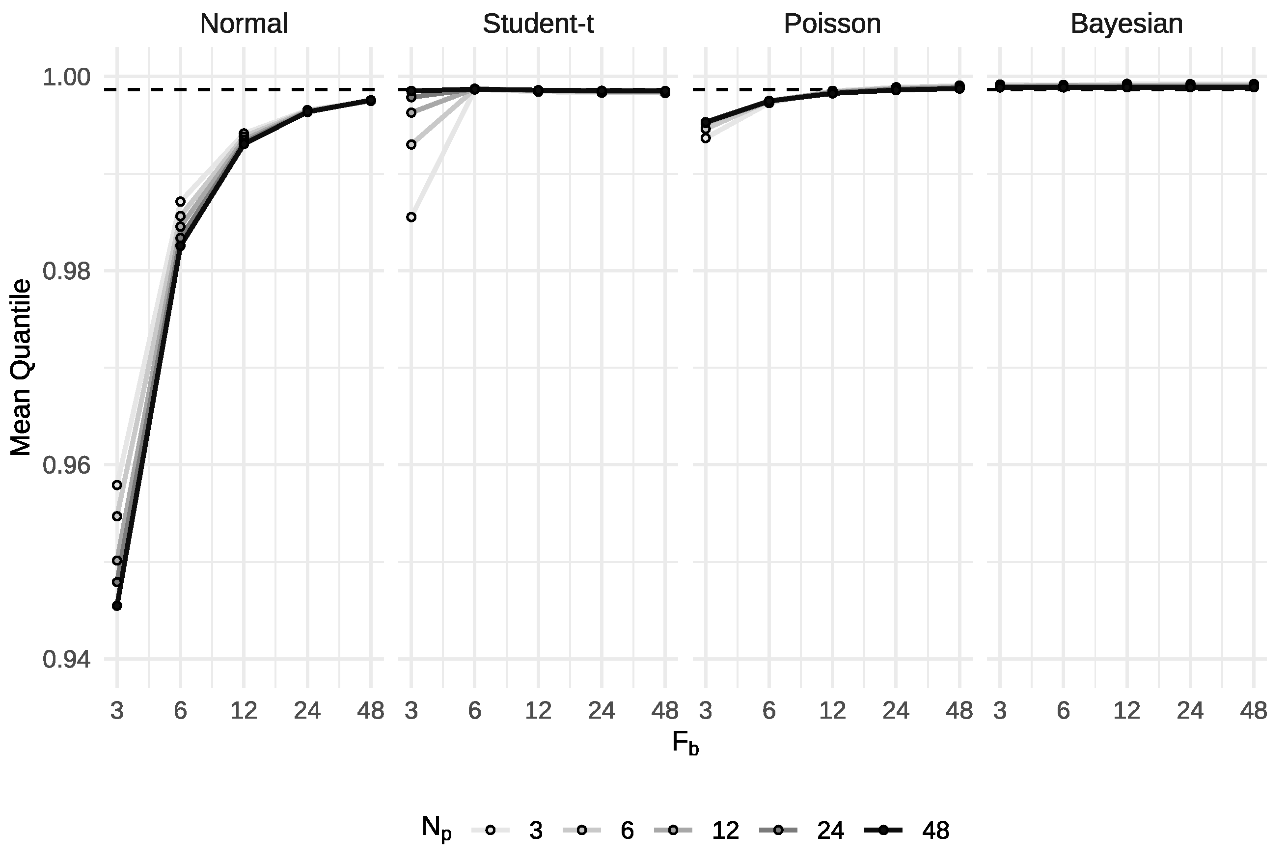
Therefore, Figure A1 shows that the Normal method can substantially underestimate the quantile (the true LOD), especially when the number of blank filters is low and the Poisson rate is high. For example, with filters, the Normal method yields an LOD corresponding to a quantile much closer to (the 2-sigma quantile) than to the nominal 3-sigma quantile ().
The Student’s t- and Poisson method can also underestimate the quantile. For the Student’s t case, the estimation becomes nearly unbiased already at , or for all when is large (e.g., ). The Poisson method is more sensitive to smaller and only approaches unbiasedness as increases. The Bayesian method slightly overestimates the quantile across the entire range.
Figure A2.
Square root of the variance in estimated quantiles vs. , by method, and by . Lower curves indicate more reproducible (less run-to-run variable) tail coverage across repeated blank studies, i.e., greater stability of the estimated detection threshold.
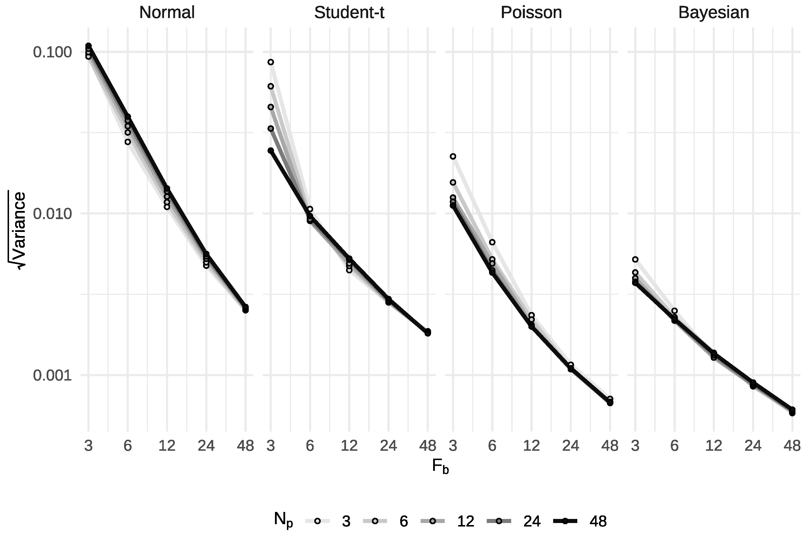
As a result, only the Bayesian method can guarantee at least the nominal 0.99865 quantile coverage for the estimated LOD across all values of and , consistently achieving or slightly exceeding the target even when the number of blank filters is small or the Poisson rate is high.
In terms of variance in Figure A2, the Normal method exhibits the highest variability in the achieved quantile across repeated blank studies, especially when the number of filters is small. This means that not only does the Normal method tend to underestimate the true LOD, but its performance is also highly inconsistent from one experiment to the next. Both the Student's t and Poisson method exhibit reduced variance compared to the Normal method, but both remain sensitive to small , with the Poisson method being particularly affected until becomes moderately large.
By contrast, the Bayesian method consistently achieves the lowest variance in quantile estimates across all combinations of and . This indicates that the Bayesian approach not only provides coverage at or only slightly above the nominal 0.99865 quantile but also delivers highly reproducible LOD estimates, minimizing run-to-run fluctuations and offering greater reliability for routine laboratory applications. Moreover, the Bayesian method can deal with situations where zero particles are observed in all filters.
References
- Hermsen, E.; Mintenig, S.M.; Besseling, E.; Koelmans, A.A. Quality Criteria for the Analysis of Microplastic in Biota Samples: A Critical Review. Environ. Sci. Technol. 2018, 52, 10230–10240. [Google Scholar] [CrossRef]
- Koelmans, A.A.; Mohamed Nor, N.H.; Hermsen, E.; Kooi, M.; Mintenig, S.M.; De France, J. Microplastics in freshwaters and drinking water: Critical review and assessment of data quality. Water Res. 2019, 155, 410–422. [Google Scholar] [CrossRef]
- Cowger, W.; Booth, A.M.; Hamilton, B.M.; Thaysen, C.; Primpke, S.; Munno, K.; Lusher, A.L.; Dehaut, A.; Vaz, V.P.; Liboiron, M.; et al. Reporting Guidelines to Increase the Reproducibility and Comparability of Research on Microplastics. Appl. Spectrosc. 2020, 74, 1066–1077. [Google Scholar] [CrossRef]
- Koelmans, A.A.; Diepens, N.J.; Mohamed Nor, N.H. Weight of Evidence for the Microplastic Vector Effect in the Context of Chemical Risk Assessment. In Microplastic in the Environment: Pattern and Process; Bank, M.S., Ed.; Environmental Contamination Remediation and Management; Springer: Cham, Switzerland, 2022; pp. 155–197. [Google Scholar] [CrossRef]
- Dawson, A.L.; Santana, M.F.; Nelis, J.L.; Motti, C.A. Taking control of microplastics data: A comparison of control and blank data correction methods. J. Hazard. Mater. 2023, 443, 130218. [Google Scholar] [CrossRef] [PubMed]
- Prata, J.C.; Padrão, J.; Khan, M.T.; Walker, T. Do’s and don’ts of microplastic research: A comprehensive guide. Water Emerg. Contam. Nanoplast. 2024, 3, 8. [Google Scholar] [CrossRef]
- IUPAC. Nomenclature, Symbols, Units and Their Usage in Spectrochemical Analysis-II. Data Interpretation. Pure Appl. Chem. 1976, 45, 99–103. [Google Scholar] [CrossRef]
- ACS Committee. Guidelines for Data Acquisition and Data Quality Evaluation in Environmental Chemistry. Anal. Chem. 1980, 52, 2242–2249. [Google Scholar] [CrossRef]
- Currie, L.A. Limits for Qualitative Detection and Quantitative Determination: Application to Radiochemistry. Anal. Chem. 1968, 40, 586–593. [Google Scholar] [CrossRef]
- Currie, L.A. Nomenclature in Evaluation of Analytical Methods including Detection and Quantification Capabilities (IUPAC Recommendations 1995). Pure Appl. Chem. 1995, 67, 1699–1723. [Google Scholar] [CrossRef]
- RSC Committee. The edge of reason: Reporting and inference near the detection limit. Anal. Methods 2020, 12, 401–403. [Google Scholar] [CrossRef] [PubMed]
- Long, G.L.; Winefordner, J.D. Limit of detection. A closer look at the IUPAC definition. Anal. Chem. 1983, 55, 712A–724A. [Google Scholar] [CrossRef]
- Mocak, J.; Bond, A.M.; Mitchell, S.; Scollary, G. A Statistical Overview of Standard (IUPAC and ACS) and New Procedures for Determining the Limits of Detection and Quantification: Application to Voltammetric and Stripping Techniques. Pure Appl. Chem. 1997, 69, 297–328. [Google Scholar] [CrossRef]
- Sijtsma, K. Never Waste a Good Crisis: Lessons Learned from Data Fraud and Questionable Research Practices; Chapman and Hall/CRC: New York, NY, USA, 2023. [Google Scholar] [CrossRef]
- Stark, P.B.; Saltelli, A. Cargo-cult Statistics and Scientific Crisis. Significance 2018, 15, 40–43. [Google Scholar] [CrossRef]
- McIntosh, R.D. Exploratory reports: A new article type for Cortex. Cortex 2017, 96, A1–A4. [Google Scholar] [CrossRef] [PubMed]
- Kerr, N.L. HARKing: Hypothesizing After the Results are Known. Personal. Soc. Psychol. Rev. 1998, 2, 196–217. [Google Scholar] [CrossRef] [PubMed]
- Nosek, B.A.; Ebersole, C.R.; DeHaven, A.C.; Mellor, D.T. The preregistration revolution. Proc. Natl. Acad. Sci. USA 2018, 115, 2600–2606. [Google Scholar] [CrossRef]
- Song, F.; Parekh, S.; Hooper, L.; Loke, Y.K.; Ryder, J.; Sutton, A.J.; Hing, C.; Kwok, C.S.; Pang, C.; Harvey, I. Dissemination and publication of research findings: An updated review of related biases. Health Technol. Assess. 2010, 14, 1–220. [Google Scholar] [CrossRef]
- Osman, A.I.; Hosny, M.; Eltaweil, A.S.; Omar, S.; Elgarahy, A.M.; Farghali, M.; Yap, P.S.; Wu, Y.S.; Nagandran, S.; Batumalaie, K.; et al. Microplastic sources, formation, toxicity, and remediation: A review. Environ. Chem. Lett. 2023, 21, 2129–2169. [Google Scholar] [CrossRef] [PubMed]
- Niari, M.H.; Ghobadi, H.; Amani, M.; Aslani, M.R.; Fazlzadeh, M.; Matin, S.; Takaldani, A.H.S.; Hosseininia, S. Characteristics and assessment of exposure to microplastics through inhalation in indoor air of hospitals. Air Qual. Atmos. Health 2025, 18, 253–262. [Google Scholar] [CrossRef]
- Li, B.; Li, M.; Du, D.; Tang, B.; Yi, W.; He, M.; Liu, R.; Yu, H.; Yu, Y.; Zheng, J. Characteristics and influencing factors of microplastics entering human blood through intravenous injection. Environ. Int. 2025, 198, 109377. [Google Scholar] [CrossRef]
- Hale, R.C.; Seeley, M.E.; King, A.E.; Yu, L.H. Analytical Chemistry of Plastic Debris: Sampling, Methods, and Instrumentation. In Microplastic in the Environment: Pattern and Process; Bank, M.S., Ed.; Environmental Contamination Remediation and Management; Springer: Cham, Switzerland, 2021; pp. 17–67. [Google Scholar] [CrossRef]
- Flyvbjerg, B.; Gardner, D. How Big Things Get Done: The Surprising Factors That Determine the Fate of Every Project, from Home Renovations to Space Exploration and Everything in Between; McClelland & Stewart: Toronto, ON, Canada, 2023. [Google Scholar]
- Rauert, C.; Charlton, N.; Bagley, A.; Dunlop, S.A.; Symeonides, C.; Thomas, K.V. Assessing the Efficacy of Pyrolysis–Gas Chromatography–Mass Spectrometry for Nanoplastic and Microplastic Analysis in Human Blood. Environ. Sci. Technol. 2025, 59, 1984–1994. [Google Scholar] [CrossRef] [PubMed]
- Rubin, M. When to adjust alpha during multiple testing: A consideration of disjunction, conjunction, and individual testing. Synthese 2021, 199, 10969–11000. [Google Scholar] [CrossRef]
- Benjamini, Y.; Heller, R. Screening for Partial Conjunction Hypotheses. Biometrics 2008, 64, 1215–1222. [Google Scholar] [CrossRef] [PubMed]
- Parker, R.A.; Weir, C.J. Non-adjustment for multiple testing in multi-arm trials of distinct treatments: Rationale and justification. Clin. Trials 2020, 17, 562–566. [Google Scholar] [CrossRef]
- Benjamini, Y.; Hochberg, Y. Controlling the False Discovery Rate: A Practical and Powerful Approach to Multiple Testing. J. R. Stat. Soc. Ser. Stat. Methodol. 1995, 57, 289–300. [Google Scholar] [CrossRef]
- Albers, C. The problem with unadjusted multiple and sequential statistical testing. Nat. Commun. 2019, 10, 1921. [Google Scholar] [CrossRef]
- Singh, A.K.; Singh, A.; Engelhardt, M. The Lognormal Distribution in Environmental Applications; Technology Support Center Issue Paper; Technical Report EPA/600/R-97/006; United States Environmental Protection Agency, Office of Research and Development, Office of Solid Waste and Emergency Response: Las Vegas, NV, USA, 1997.
- Limpert, E.; Stahel, W.A.; Abbt, M. Log-normal Distributions across the Sciences: Keys and Clues. BioScience 2001, 51, 341–352. [Google Scholar] [CrossRef]
- Razali, N.M.; Wah, Y.B. Power comparisons of Shapiro-Wilk, Kolmogorov-Smirnov, Lilliefors and Anderson-Darling tests. J. Stat. Model. Anal. 2011, 2, 21–33. [Google Scholar]
- Taagepera, R. Ignorance-Based Quantitative Models and Their Practical Implications. J. Theor. Politics 1999, 11, 421–431. [Google Scholar] [CrossRef]
- Fenton, L.F. The sum of log-normal probability distributions in scatter transmission systems. Ire Trans. Commun. Syst. 1960, 8, 57–67. [Google Scholar] [CrossRef]
- Zhang, Y.; Kwok, Y.K. Saddlepoint approximations to tail expectations under non-Gaussian base distributions: Option pricing applications. J. Appl. Stat. 2020, 47, 1936–1956. [Google Scholar] [CrossRef]
- Chernoff, H. A measure of asymptotic efficiency for tests of a hypothesis based on the sum of observations. Ann. Math. Stat. 1952, 23, 493–507. [Google Scholar] [CrossRef]
- Arivazhahan, A. Principles of EC50, ED50, pD2 and pA2 Values of Drugs. In Introduction to Basics of Pharmacology and Toxicology; Springer: Berlin/Heidelberg, Germany, 2022; pp. 143–156. [Google Scholar] [CrossRef]
- Kazakova, R.R.; Masson, P. Quantitative Measurements of Pharmacological and Toxicological Activity of Molecules. Chemistry 2022, 4, 1466–1474. [Google Scholar] [CrossRef]
- Ruxton, G.D. The unequal variance t-test is an underused alternative to Student’s t-test and the Mann–Whitney U test. Behav. Ecol. 2006, 17, 688–690. [Google Scholar] [CrossRef]
- Chernick, M.R. Bootstrap Methods: A Guide for Practitioners and Researchers, 2nd ed.; Wiley Series in Probability and Statistics; John Wiley & Sons: Hoboken, NJ, USA, 2011. [Google Scholar]
- Meeker, W.Q.; Hahn, G.J.; Escobar, L.A. Statistical Intervals: A Guide for Practitioners and Researchers, 2nd ed.; John Wiley & Sons: Hoboken, NJ, USA, 2017. [Google Scholar]
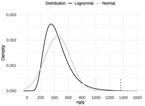
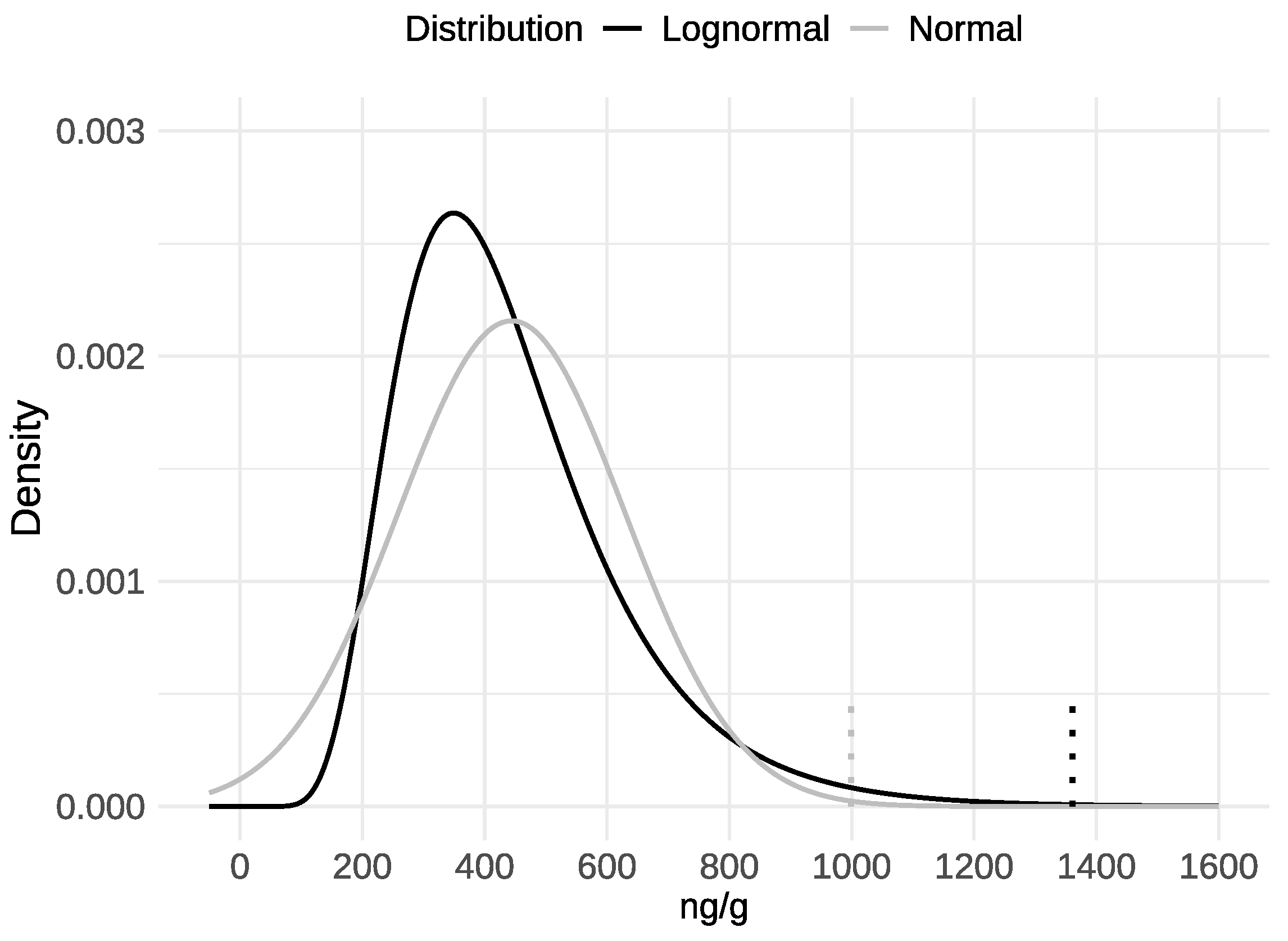
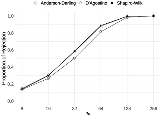
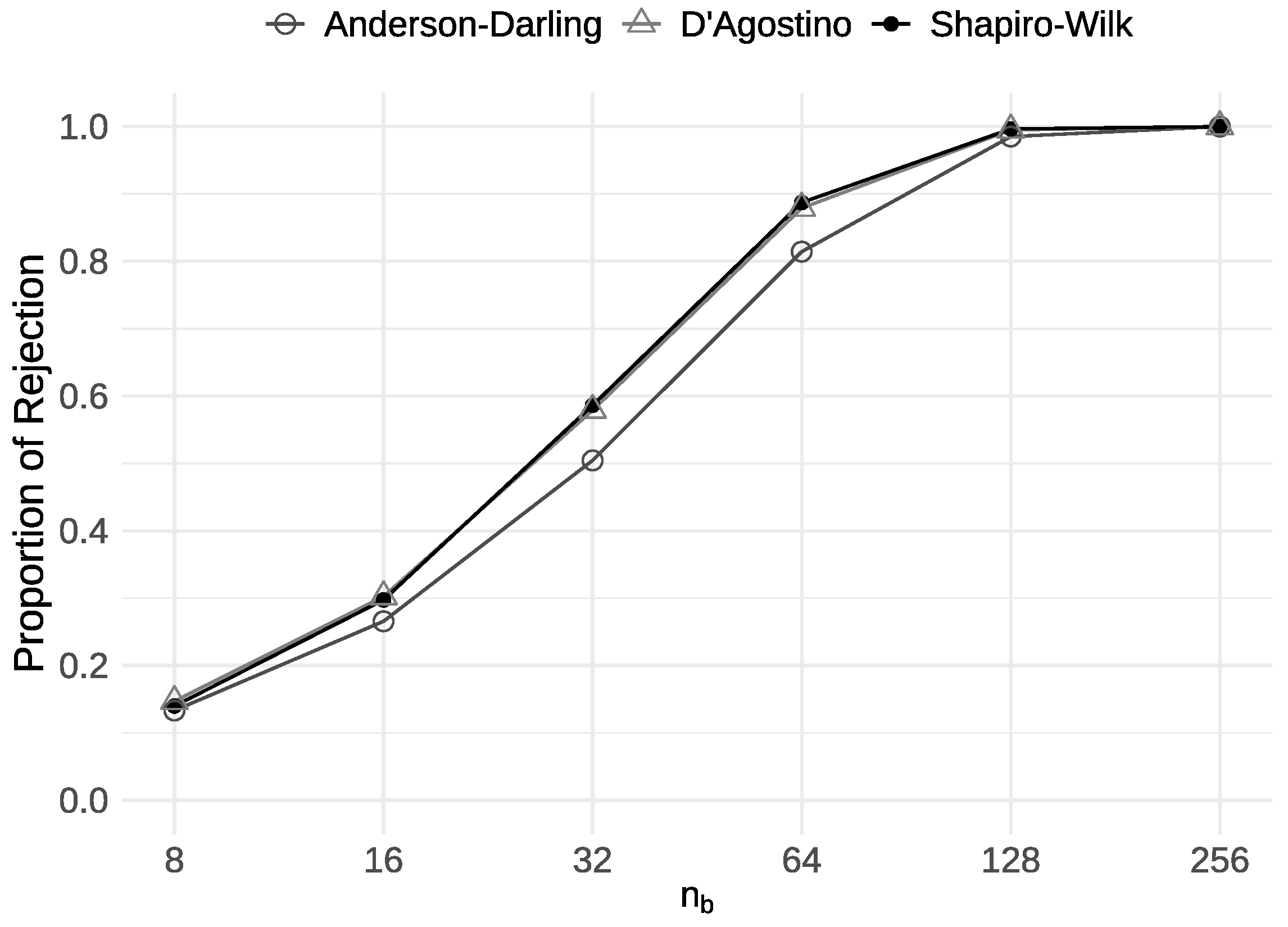
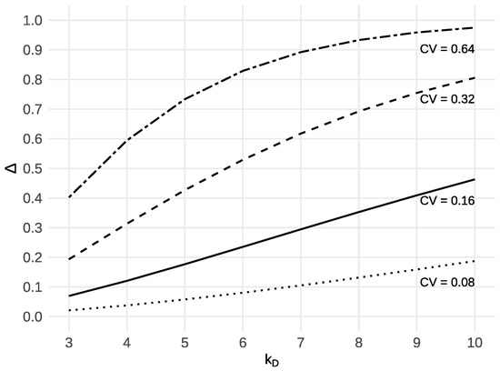
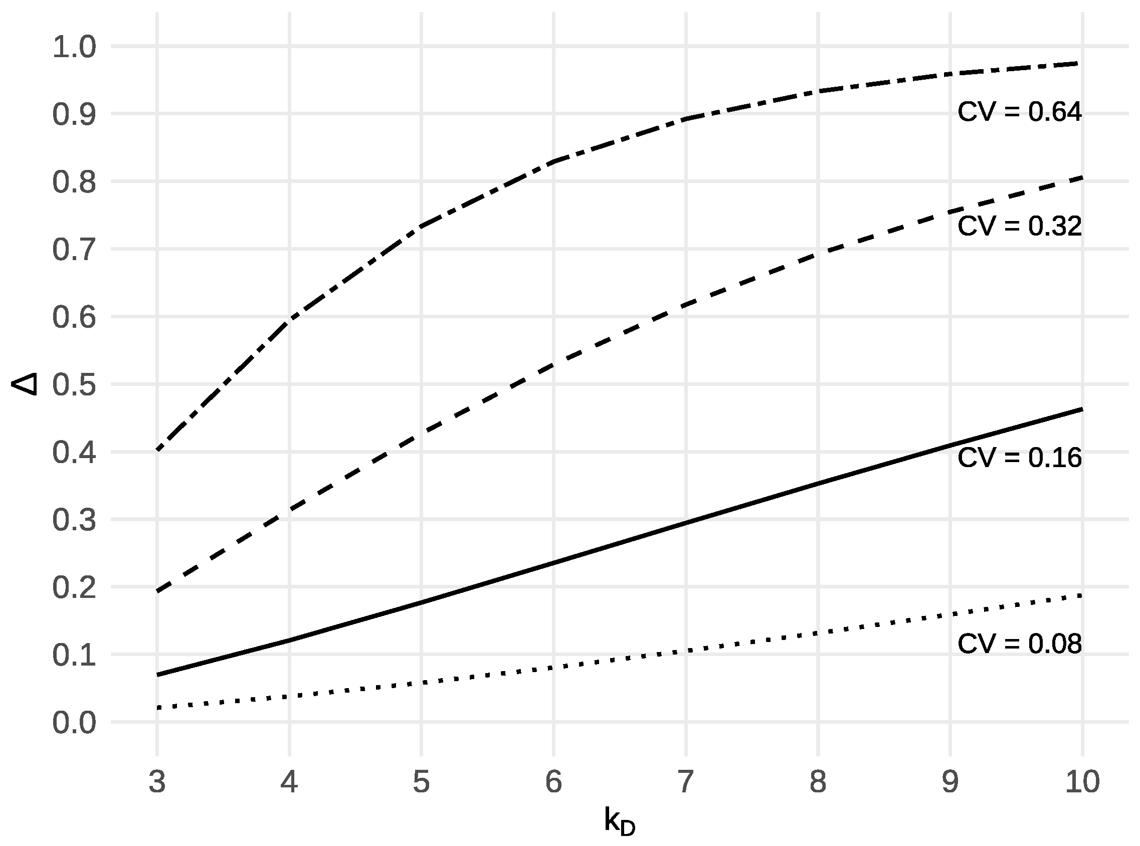
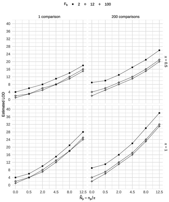
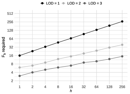

Disclaimer/Publisher’s Note: The statements, opinions and data contained in all publications are solely those of the individual author(s) and contributor(s) and not of MDPI and/or the editor(s). MDPI and/or the editor(s) disclaim responsibility for any injury to people or property resulting from any ideas, methods, instructions or products referred to in the content. |
© 2026 by the authors. Licensee MDPI, Basel, Switzerland. This article is an open access article distributed under the terms and conditions of the Creative Commons Attribution (CC BY) license.