A Tropospheric Delay Model for InSAR in Alpine Canyon Regions Through Incorporation of Time-Varying Gaussian Coefficients and Coupled ZWD

Abstract

This study addresses the stratified and turbulent tropospheric delays that impede interferometric synthetic aperture radar (InSAR) deformation monitoring in alpine canyon regions. We introduce a tropospheric delay model that incorporates time-varying Gaussian coefficients and coupled zenith wet delay (ZWD) by combining diverse multi-source data. This model was incorporated into StaMPS for InSAR processing. Evaluation results demonstrated that (1) the model accurately captured seasonal and diurnal tropospheric variations, achieving a root mean squared error (RMSE) of 2.01 cm relative to the GNSS reference data; (2) the model corrected stratified and turbulent delays and reduced interferometric phase standard deviation (STD) by 9.28% compared to the Generic Atmospheric Correction Online Service (GACOS); and (3) the deformation accuracy improved by 19.07% over GACOS. Discussion results indicate that accounting for time-varying Gaussian coefficients is essential and that coupling ZWD to rectify turbulent delays outperformed the filtering method. The observed negative interferogram corrections result from the random intensity of turbulent delays. These findings confirm the effectiveness of the proposed model for high-precision InSAR deformation monitoring in complex alpine terrains. The proposed model aims to enhance studies of tropospheric delay variations in alpine canyon regions and to mitigate such delays in InSAR-based geological hazard monitoring.

1. Introduction

Northwest Yunnan Province, China, possesses a complex geological structure with numerous active faults and a humid climate marked by heavy rainfall, resulting in fractured and unstable rock strata. Consequently, the area is highly susceptible to landslides, posing severe threats to population and property safety and presenting significant challenges for disaster prevention and control.

Although national initiatives have prioritized geological disaster prevention, the unique geology and climate of the region have rendered most events beyond existing early-warning systems, as evidenced by the Fugong landslide on 18 March 2025. Accurately detecting the timing and location of geological disasters remains critically urgent.

Surface deformation monitoring is a fundamental method for identifying geological hazards, with conventional techniques including GNSS, leveling measurements, LiDAR, and hydrogeological analysis [1]. However, these methods are limited in achieving large-scale, high spatiotemporal resolution deformation monitoring due to high resource demands and restricted sampling density. In contrast, interferometric synthetic aperture radar (InSAR) offers all-weather, global coverage with high spatial resolution, whereas traditional geodetic techniques provide only sparse observations. InSAR has become indispensable for examining precursory deformation characteristics associated with hazards, including landslides, earthquakes, volcanic activity, and ground subsidence [2,3,4].

Differential InSAR (D-InSAR) determines surface deformation by subtracting the terrain phase from the observation phase. Researchers have utilized D-InSAR to monitor surface deformations related to earthquakes, volcanic movements, glacier dynamics, plate tectonics, mining activities, and groundwater extraction [5,6,7,8]. To address spatiotemporal incoherent noise and atmospheric delays, time series InSAR (TS-InSAR) techniques evolved from D-InSAR [9,10,11]. Two prominent TS-InSAR methods are permanent scatterers (PS) and the small baseline subset (SBAS) [12,13]. Hooper et al. developed the Stanford method for PS (StaMPS), which eliminates spatially correlated phase noise to identify stable scatterers, thereby increasing PS densities [14]. Subsequently, Ferretti et al. introduced distributed scatterers InSAR (DS-InSAR), which combines PS and distributed scatterers approaches to increase the measurement point (MP) density in vegetated, mountainous regions like Northwest Yunnan [15].

Despite advancements, InSAR measurements continue to be influenced by terrain, orbital, and decorrelation errors, with atmospheric error being the predominant factor [16]. Atmospheric effects originate in both the ionosphere and troposphere. While ionospheric effects significantly impact P-band and L-band SAR data, their influence on C-band Sentinel-1A SAR data is negligible [17,18,19]. Zenith tropospheric delay (ZTD), the delay along the zenith, comprises zenith hydrostatic delay (ZHD) and zenith wet delay (ZWD). ZHD results from air pressure and temperature, whereas ZWD arises from water vapor. ZTD can also be decomposed into stratified and turbulent delay based on the physical mechanism of its generation. InSAR measurements are affected by both stratified and turbulent delays. Stratified delay, related to the electromagnetic wave propagation path, corresponds to ZTD and significantly impacts deformation results over undulating terrain due to the dependence of InSAR measurements on spatial geometry. Stratified delay often exhibits seasonal variations [20,21,22], with phase differences induced by stratified delay potentially exceeding 10 mm for height variations of 500 m [23]. Turbulent delay, primarily caused by lateral variations or irregular motions in the troposphere, occurs both over flat and mountainous terrain. It is typically visible more on flat areas where the stratified delay component is not dominant [24]. Northwest Yunnan, characterized by severe terrain undulations and a complex climate, is an alpine canyon region where InSAR measurements are simultaneously influenced by seasonal stratified delay from terrain undulations and by turbulent delay due to water vapor fluctuations [25]. These combined effects can lead to erroneous inversions or the masking of genuine deformation [26]. Seasonal variations in tropospheric delay, averaging 10 cm, can induce deformation errors of up to 23.8 cm [27]. Therefore, the precise correction of both stratified and turbulent delays is imminent.

Correction methodologies are categorized into three types: statistical, empirical, and predictive. The statistical approach (e.g., filtering and stacking) is limited, as it presumes atmospheric effects vary randomly over time [28]. Empirical techniques (e.g., linear and power-law models) mitigate stratified delay by modeling the relationship between InSAR phase and terrain. However, their performance declines when turbulent delays dominate or when deformation signals correlate with terrain [29,30]. The power-law method, which accounts for atmospheric spatial variability, is applicable to interferograms exhibiting terrain-related deformations [31]. While statistical and empirical methods rely on interferogram phase data, predictive approaches utilize external atmospheric information to estimate and correct tropospheric delay [32,33]. Nonetheless, predictive methods face challenges related to the spatiotemporal resolution and accuracy of external data models. The Generic Atmospheric Correction Online Service (GACOS) exemplifies a predictive method. GACOS computes atmospheric delay with a spatial resolution of 0.125° and a temporal resolution of six hours, utilizing high-resolution European Centre for Medium-Range Weather Forecasts (HRES-ECMWF) data [34]. The resulting zenith delays are projected onto the line-of-sight (LOS) and spatially densified to 90 m, matching the interferogram pixel spacing via an iterative tropospheric-decomposition spatial interpolator [35]. GACOS distinguishes between stratified and turbulent delays, both of which are examined in detail in this study.

The analysis explores the statistical properties and spatial variability of each component across diverse terrains, highlighting their implications for InSAR time-series analysis. For turbulent delay, GACOS employs an inverse distance weight (IDW) interpolator, while stratified delay follows an exponential distribution [36]. This decomposition allows for customized correction strategies tailored to each component. Challenges include errors inherent in the HRES-ECMWF dataset, its relatively coarse spatial resolution, and temporal discrepancies between meteorological fields and SAR acquisitions, which can introduce artifacts into deformation estimates. Yu et al. proposed a workflow that uses GACOS to correct long-wavelength tropospheric delay and satisfy InSAR time-series analysis assumptions, subsequently applying spatiotemporal filters to eliminate short-wavelength residuals [37]. Zhang et al. integrated GACOS with principal component analysis (PCA) to rectify tropospheric delay within an SBAS-InSAR framework, using PCA to process residual delays after GACOS [38].

Separating the corrections for stratified and turbulent delays remains the mainstream approach, employing distinct strategies based on the characteristics of each component to minimize the overall tropospheric impact. A method utilizing quadtrees to adaptively control tropospheric spatial variability was proposed. This approach incorporates tropospheric delay, deformation, and terrain error into a unified model, subsequently isolating terrain-related tropospheric delay [39]. Murray et al. found that integrating a linear model with weather model products can capture subtle signals [40]. The calculation of ZTD using ERA5 data has garnered significant attention [41,42]. Guo et al. developed a periodic ZTD negative exponential function (PZTD-NEF) model, accounting for atmospheric spatiotemporal variations derived from the fifth-generation ECMWF atmospheric reanalysis (ERA5). This model reduced seasonal oscillations of stratified delay and enhanced deformation time series accuracy by 40.04% [43]. However, the nonlinear temporal characteristics of tropospheric delay may surpass anticipated seasonal oscillations. To address this, Guo et al. introduced the Prophet-ZTD-NEF model [44]. Additionally, researchers have explored turbulent delay correction. One team integrated a spatial stochastic troposphere model with a weighted strategy to correct turbulent delay [45,46].

Current correction methods concentrate solely on stratified or turbulent delay, leading to residual tropospheric errors. Comprehensive approaches that tackle both delays have yet to develop detailed models based exclusively on their distinct characteristics, thereby hindering accurate estimation. Developing a high-precision tropospheric delay model within the complex environment of Northwest Yunnan presents an urgent challenge.

Northwest Yunnan plays a crucial role in geological disaster prevention and control, necessitating the use of InSAR technology for deformation monitoring. Stratified and turbulent delays coexist in Northwest Yunnan, attributed to its undulating terrain and three-dimensional climate. Effective InSAR application in alpine canyon regions requires addressing two key issues: correcting terrain-induced seasonal stratified delays and compensating for turbulent delays caused by water vapor variations. The primary challenge in addressing the first issue lies in mitigating the seasonal oscillations of stratified delays, while the second issue requires accurately characterizing the variation in turbulent delays. In this study, we propose an InSAR tropospheric delay model that incorporates time-varying Gaussian coefficients and coupled ZWD, integrating it into StaMPS for processing. The model seeks to simultaneously mitigate stratified and turbulent delays in alpine canyon regions, thereby producing high-precision deformation results. The proposed model is expected to offer valuable guidance for geological hazard monitoring and early warning, as well as serve as a foundation for compiling and updating the geological hazard inventory in Northwest Yunnan.

The remainder of this article is organized as follows: Section 2 presents the materials and methods, while Section 3 evaluates the effectiveness of the proposed model in mitigating interferogram tropospheric delay and assessing deformation accuracy. We discuss the necessity of considering the time-varying Gaussian coefficients and the influence factors of coupling ZWD to correct the turbulent delay in Section 4. Lastly, the conclusions of the study are summarized in Section 5.

2. Materials and Methods

2.1. Study Area

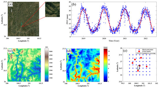
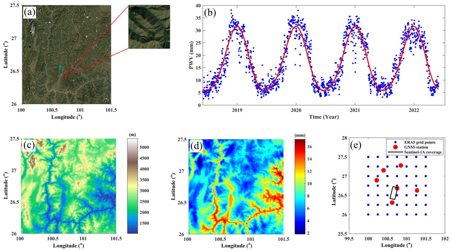
The research focuses on an alpine canyon in Northwest Yunnan Province, China, where active atmospheric conditions notably impact InSAR measurements due to tropospheric delay. Figure 1a,c illustrate the study area’s latitude range of 26° N–27.5° N and its undulating terrain, with elevations spanning from 1015 m to 5397 m. Figure 1b,d show the seasonal variability of precipitable water vapor (PWV), ranging from approximately 5 mm in winter to 30 mm in summer, highlighting significant seasonal fluctuations driven by the region’s complex topography. The pronounced contrast between winter and summer PWV emphasizes the role of seasonal atmospheric dynamics. As previously mentioned, InSAR is vulnerable to stratified delays caused by topographic variations and turbulent delays resulting from PWV fluctuations. Accurately estimating both stratified and turbulent delays in alpine canyon regions presents considerable challenges, justifying its selection for this investigation.

Figure 1. (a) Image of the study area. (b) PWV time series. (c) DEM. (d) PWV distribution. (e) Data distribution.

Figure 1e displays ERA5 grid points (blue), GNSS stations providing ZTD measurements (red), and Sentinel-1A coverage (black box). These data sources offer complementary insights, with ERA5 providing gridded reanalysis and GNSS stations delivering in situ ZTD observations. This study utilizes ERA5 and GNSS ZTD data to examine the spatiotemporal characteristics of ZTD and to develop a robust ZTD model. The interferograms derived from SAR data aid in determining the surface deformation velocities and time series.

2.2. Data

ERA5 atmospheric reanalysis data, with a horizontal resolution of 0.25° × 0.25° and hourly temporal resolution, represent the latest ERA series products. ERA5 provides both surface variables—including temperature, pressure, dew-point temperature, and precipitable water vapor (PWV)—and data across 37 standard pressure levels, comprising temperature, pressure, specific humidity, and geopotential. Due to its global coverage and accessibility, ERA5 has become a crucial resource for atmospheric research. Zhang et al. evaluated ERA5 for InSAR tropospheric delay correction across various seasons, climate zones, and terrains, demonstrating that ERA5 fulfills InSAR delay-correction requirements [47]. ERA5 was used as the data resource for modeling in this study.

GNSS offers automated, all-weather, high-precision navigation and positioning, time–frequency signals, surface deformation, and tropospheric parameters. GNSS ZTD and surface displacement derived via GAMIT software (Version 10.5) often serve as reference data given their accuracy [48,49]. Six GNSS stations (Figure 1e) provided ZTD, while the stations used for surface displacement are indicated subsequently. GNSS was used as the data resource for modeling and verifying the model in this study.

In this study, 75 C-band Sentinel-1A SAR images from 22 March 2019 to 20 October 2022 were preprocessed to generate interferograms with GAMMA software (Version 20160701). Sentinel-1A has a pixel spacing of 2.3 m in range and 13.9 m in azimuth. Sentinel-1A data, due to rapid acquisition, have been widely utilized in detecting and analyzing land deformation, landslides, earthquakes, volcanic activity, and other geohazards using TS-InSAR technology [50,51,52].

2.3. Methods

The fundamental observation—interferograms—represents the phase difference between two acquisitions. The interferometric phase is expressed as follows:

$$\mathrm{\varnothing }={\mathrm{\varnothing }}_{def}+{\mathrm{\varnothing }}_{stra}+{\mathrm{\varnothing }}_{turb}+{\mathrm{\varnothing }}_{dem}+{\mathrm{\varnothing }}_{orb}+{\mathrm{\varnothing }}_{noi}$$

(1)

where ${\mathrm{\varnothing }}_{def}$ denotes the deformation phase along the LOS, ${\mathrm{\varnothing }}_{stra}$ and ${\mathrm{\varnothing }}_{turb}$ represent the stratified and turbulent atmospheric delay phases, ${\mathrm{\varnothing }}_{dem}$ arises from topographic errors, ${\mathrm{\varnothing }}_{orb}$ from orbital inaccuracies, and ${\mathrm{\varnothing }}_{noi}$ from pixel scattering variability. A 30 m resolution Shuttle Radar Topography Mission Digital Elevation Model (SRTM DEM) corrected topographic errors, while precise orbit files addressed orbital inaccuracies. A filtering algorithm reduced noise. This study focuses on correcting stratified and turbulent delays in InSAR measurement.

InSAR-derived displacements are relative between measurement points (MPs) and the chosen unwrapping reference point due to spatial relativity. Stratified delay in InSAR measurement is caused by the height difference between the MPs and the reference point. It is typically more visible in alpine canyon regions.

ERA5 atmospheric reanalysis data were employed to calculate the ZTD using the following integral method:

$$\mathrm{Z}\mathrm{T}\mathrm{D}={10}^{-6}{\int }_{h_{\mathrm{s}\mathrm{u}\mathrm{r}\mathrm{f}}}^{h_{\mathrm{t}\mathrm{o}\mathrm{p}}}N\mathrm{d}H$$

(2)

$$N={\displaystyle \frac{k_1\left(P-e\right)}{T}}+{\displaystyle \frac{k_{2}e}{T}}+{\displaystyle \frac{k_{3}e}{T^2}}$$

(3)

$$e={\displaystyle \frac{Sh·P}{0.622}}$$

(4)

where $h_{\mathrm{s}\mathrm{u}\mathrm{r}\mathrm{f}}$ and $h_{\mathrm{t}\mathrm{o}\mathrm{p}}$ represent the Earth’s surface height and troposphere top height, N denotes the total refractivity, H denotes the height, $k_1$, $k_2$, and $k_3$ indicate the refractive constants, P denotes pressure, e represents the water vapor pressure, T indicates the temperature, and $Sh$ denotes the specific humidity.

The Saastamoinen model estimated the ZHD at the tropopause, which was used to correct the integrated ZTD [53]. The formula is expressed as follows:

$${ZHD}_{top}={\displaystyle \frac{0.0022767·P_{top}}{1-0.002667·\mathit{cos}\left(2\phi \right)-0.00000028·h_{top}}}$$

(5)

where ${ZHD}_{top}$ represents the ZHD at the troposphere top, $P_{top}$ denotes the pressure at the troposphere top, and φ indicates the latitude.

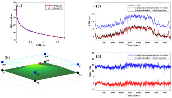
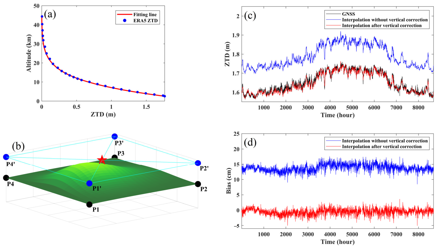
Figure 2a displays vertical ZTD variations as blue points, indicating an increase in ZTD with decreasing altitude. Accurately determining ZTD at the target point necessitates adjusting for altitude differences between surrounding points and the target, a process that can introduce substantial errors. In our previous research [54], the Gaussian function demonstrated superior performance in modeling these vertical ZTD variations. Consistently, this study adopts the same methodology. The red curve in Figure 2a represents the Gaussian fit.

Figure 2. (a) Vertical variation and fitting line of ZTD. (b) Interpolation process. (c) Interpolation results without vertical correction and after vertical correction. (d) Bias of interpolation without vertical correction and after vertical correction. Note that the black points in (b) represent the position before vertical correction, the blue points represent the position after vertical correction, and the red star represents the target point.

Figure 2b illustrates the interpolation process for the target ZTD point using four adjacent grid points. After vertical correction, the results closely aligned with GNSS observations, whereas uncorrected biases exceeded 10 cm (Figure 2c,d). Therefore, vertical correction for ZTD is imperative. The formula for vertical correction is given by Equation (6) as follows:

$${ZTD}_t={ZTD}_s·e^{\left[{\displaystyle \frac{{\left(H_s-b\right)}^2-{\left(H_t-b\right)}^2}{c^2}}\right]}$$

(6)

where $H_{\mathrm{s}}$ and $H_{\mathrm{t}}$ represent the starting and target heights, ${ZTD}_s$ and ${ZTD}_t$ denote the ZTD at $H_{\mathrm{s}}$ and $H_{\mathrm{t}}$, and b and c represent the Gaussian coefficients, respectively.

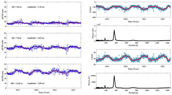
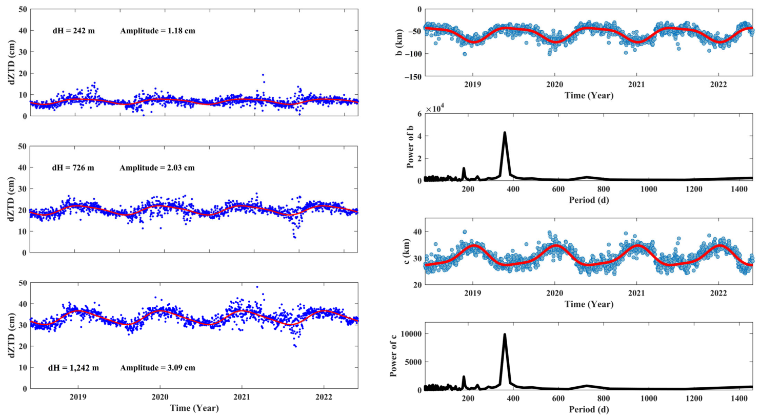
These findings underscore the critical importance of elevation-dependent corrections in ensuring ZTD consistency with GNSS data. Furthermore, the amplitude of differential ZTD (dZTD) varies with the differential height (dH) between two points. Four GNSS stations with elevations of 1204 m, 1446 m, 1930 m, and 2446 m were selected to visualize the variations, and the first station was used as the reference point. As depicted in the first column of Figure 3, amplitudes of 1.18, 2.03, and 3.09 cm correspond to dH of 242, 726, and 1242 m, respectively. Consequently, larger height disparities between the unwrapping point and MPs result in more pronounced seasonal effects. This behavior highlights the significance of height differentials in seasonal ZTD modeling. In our previous study [54], we developed a ZTD model incorporating annual, semiannual, diurnal, and semidiurnal periods. The current study employs the same approach to construct the ZTD model. Additionally, the Gaussian coefficients b and c in Equation (6) were time-variant rather than constant. The second column of Figure 3 presents their time series and corresponding Fourier transforms, which reveal annual and semiannual variations. To mitigate seasonal impacts, we developed a time-varying Gaussian coefficient model as described in Equation (7) as follows:

$$\begin{array}{c}cof={\alpha }_0+{\alpha }_{1}cos\left(2\pi {\displaystyle \frac{doy}{365.25}}\right)+{\alpha }_{2}sin\left(2\pi {\displaystyle \frac{doy}{365.25}}\right)+{\alpha }_{3}cos\left(4\pi {\displaystyle \frac{doy}{365.25}}\right)\hfill \\ +{\alpha }_{4}sin\left(4\pi {\displaystyle \frac{doy}{365.25}}\right)\hfill \end{array}$$

(7)

where $cof$ denotes the Gaussian coefficient b or c, ${\alpha }_0$ indicates the mean value of Gaussian coefficients, ${\alpha }_1$–${\alpha }_4$ represent the period amplitude coefficients, and doy indicates the day of the year.

Figure 3. The first column is the time series of ZTD with different height differences. The second column is the time series of Gaussian coefficients b and c and their Fourier transform. Note that the red line represents the fitting line.

This model explicitly accounts for temporal variability in Gaussian coefficients. The following section discusses the necessity of incorporating time-varying effects of Gaussian coefficients in ZTD estimation. In our previous study, the ZTD model was constructed using standalone ERA5 reanalysis data on a coarse grid with a spatial resolution of 0.25° × 0.25° (longitude × latitude). To improve this framework, both ERA5 and GNSS data are integrated to resolve the ZTD and Gaussian coefficients at a spatial resolution of 30 m, followed by the IDW interpolator to estimate the ZTD at the MPs.

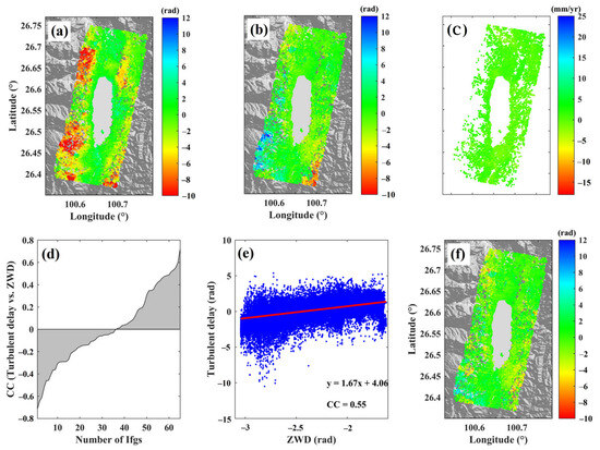
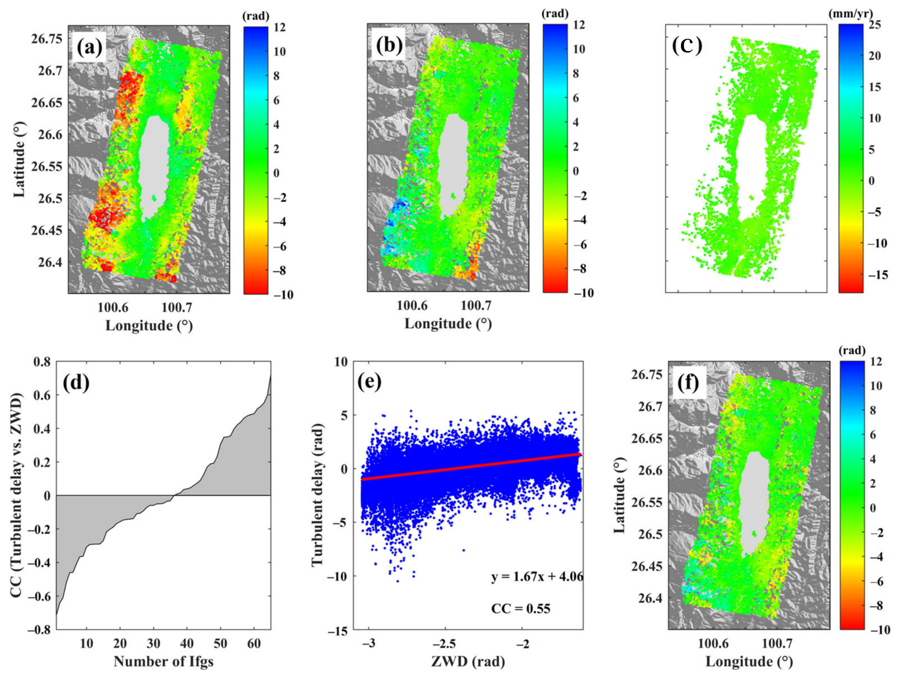
The stratified delay can be corrected using the above procedure. For example, the 12-day time-baseline interferogram illustrates the correction of tropospheric delay. After correcting for terrain and other errors, the interferogram phase contained only stratified and turbulent delays, free from deformation due to the short baseline. Figure 4a,b show the original interferogram stratified-delay subtraction from the original interferogram, respectively. The phase standard deviation (STD) decreased from 2.31 rad (a) to 1.39 rad (b); however, random noise remained, indicating the influence of turbulent delay. STD serves as a criterion for tropospheric delay mitigation and will be examined subsequently. Although stratified delay constitutes the majority of tropospheric delay in alpine canyon regions, turbulent delay caused by complex climate and abundant water vapor cannot be neglected. This study investigated the relationship between turbulent delay and ZWD because turbulent delay primarily depends on atmospheric wet components. We masked deformation points to prevent the influence of long-baseline deformation phases before analyzing the turbulent delay–ZWD relationship. LOS deformation velocities exceeding 2 mm/yr are considered unstable for C-band Sentinel-1A data [20]. Figure 4c shows the masking of points with initial LOS deformation velocities exceeding 2 mm/yr. Figure 4d shows the correlation coefficient (CC) between turbulent delay and ZWD for 65 interferograms spanning different seasons. The relationship between the correction performance of turbulent delay and CC for these interferograms has been discussed in Section 4. Figure 4e presents the linear relationship between turbulent delay and ZWD after masking, as follows:

$$D_{turb}=k·ZWD+c_0$$

(8)

where $D_{turb}$ denotes the turbulent delay, k indicates the slope, ZWD represents the zenith wet delay, and $c_0$ denotes a constant.

Figure 4. An example of correcting the stratified and turbulent delays for an original interferogram. (a) Original interferogram. (b) After correcting the stratified delay. (c) The mask results. (d) CC of 65 interferograms. (e) The relationship between turbulent delay and ZWD. Note that the red line is the fitting result (f) After correcting the turbulent delay.

Notably, ERA5 provides both ZTD and ZWD parameters. The wet refractivity formula is given by the following equation:

$$N_w=k_2^{\prime }{\displaystyle \frac{e}{T}}+k_3{\displaystyle \frac{e}{T^2}}$$

(9)

where $k_2^{\prime }$ represents the refractive constant. Substituting $N_w$ into (2) yields ERA5 ZWD. The ZWD at MPs is obtained using the same method as ZTD. It is then converted to turbulent delay at MPs using (8). Note that GNSS ZWD is obtained by subtracting ZHD from ZTD, and ZHD is calculated using (5). The total tropospheric delay was obtained by summing the stratified and turbulent delays. Figure 4f displays the interferogram after correcting for turbulent delay; the STD decreased to 1.24 rad, indicating a reduction in random noise.

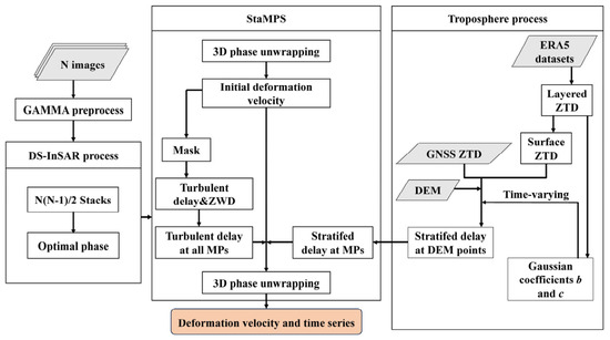
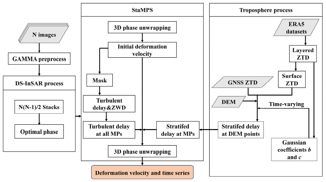
This method was integrated into the StaMPS framework to ensure accurate InSAR deformation retrieval by correcting for stratified and turbulent delays. This study employed DS–InSAR due to its ability to utilize distributed scatterers and its advantages over PS–InSAR and SBAS–InSAR in mountainous regions. Figure 5 outlines the workflow of the proposed tropospheric delay correction model for InSAR. GAMMA software preprocessed the N SAR images. We first identified MPs based on the amplitude dispersion index. Since DS can be affected by decorrelation noise, it is necessary to optimize the phase of DS. Subsequently, we used a temporal phase optimization algorithm based on the principle of phase triangulation (PT) to process N(N − 1)/2 interferometric stacks sequentially to generate the optimized phase. The optimized phase facilitated the determination of initial deformation velocity through 3D phase unwrapping with the coherence threshold set to 0.5. Tropospheric processing is the core component of the workflow for tropospheric delay correction. Layered ZTD, representing ZTD profiles at various altitudes, was obtained by integrating meteorological parameters from ERA5. The layered ZTD was modeled using a Gaussian function, yielding coefficients b and c. Subsequently, a time-varying Gaussian coefficient model was developed. Surface ZTD, defined at the Earth’s surface, was extracted from the layered ZTD. ZTD values at DEM points with a 30 m resolution were interpolated using the IDW method by incorporating GNSS data and surface ZTD, which were vertically corrected using the Gaussian coefficient model, and then ZTD values at MPs were obtained. After correcting the original interferograms for stratified delay, the turbulent delay was determined. ZWD acquisition employed the same method as for ZTD. Points with initial deformation velocities exceeding 2 mm/yr were masked. A linear relationship between turbulent delay and ZWD was established at the remaining points, enabling the estimation of turbulent delay at all MPs. The 3D phase unwrapping algorithm was reapplied to derive deformation velocities and time series after correcting for the stratified and turbulent delays in the interferograms.

Figure 5. Workflow of the proposed method. Note that the gray box represents input data and the orange box represents output data.

3. Results

The performance of the proposed model is evaluated in terms of the accuracy of the model-derived ZTD at GNSS stations, the effectiveness of the correction of the tropospheric delay within individual interferograms, the accuracy of the estimated deformation velocities, and the accuracy of the retrieved time-series deformation.

3.1. Evaluation of the Tropospheric Delay Model Estimation Performance

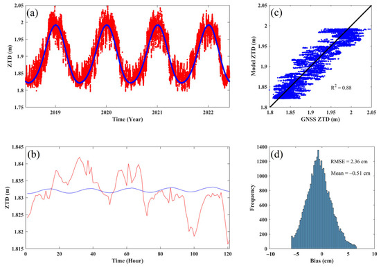
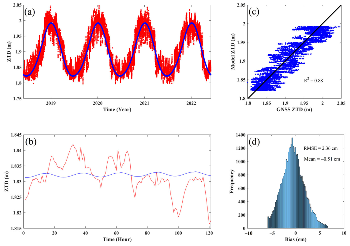
Assessing the performance of the model in estimating tropospheric delay prior to InSAR application was essential. Model accuracy for hourly tropospheric delay was validated against GNSS ZTD data from 2019 to 2022. The Leave-One-Out Cross Validation (LOOCV) was adopted to evaluate model accuracy. Specifically, when validating the model accuracy at any given GNSS station, the data from the remaining five GNSS stations were utilized for the modeling process. In Figure 6a,b, ZTD varied by approximately 15 cm annually and 1 cm daily, reflecting seasonal and diurnal variations. Seasonal fluctuations surpassed diurnal variations; nonetheless, the 1 cm diurnal change warrants attention. The proposed model simultaneously captured seasonal and diurnal ZTD variations, demonstrating superior performance in seasonal trends. It replicated the daily ZTD pattern but did not achieve optimal fitting, likely due to limitations of the trigonometric functions used. Figure 6c shows the correlation between the model and GNSS ZTD with R² = 0.88. Figure 6d depicts the bias distribution, where bias values further from zero occur less frequently. The model exhibited an RMSE of 2.01 cm and a mean bias of −0.51 cm. RMSE values at the other five GNSS stations were 2.29, 2.70, 1.93, 2.03, and 2.40 cm, resulting in an average RMSE of 2.23 cm. This assessment confirmed the capability of the model to estimate ZTD with high precision. The model applied for ZTD correction of InSAR interferograms was developed using data from all six GNSS stations.

Figure 6. Accuracy estimation for the proposed model using GNSS ZTD. (a) Seasonal variation of ZTD. (b) Relationship between model ZTD and GNSS ZTD. (c) Diurnal variation of ZTD. (d) Frequency of bias. Note that red markers in (a) and lines in (b) represent ZTD at the same GNSS station, while blue lines indicate model ZTD.

3.2. Overall Evaluation of Correcting Tropospheric Delay for Interferograms

Prior to tropospheric delay correction, quality control of 75 Sentinel-1A SAR interferograms was implemented to reduce meteorological artifacts. Xiao et al. employed cross-validation to exclude “bad” interferograms, retaining only the “good” cases [55].

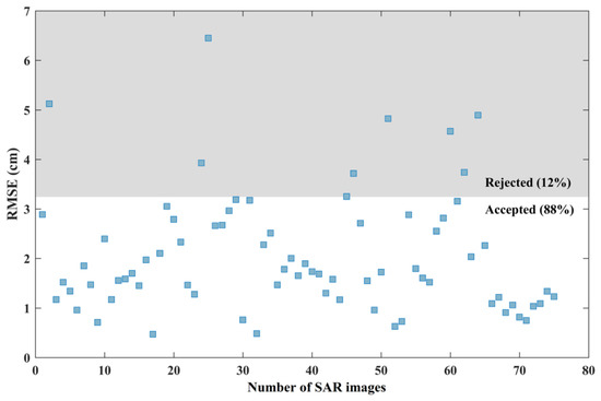
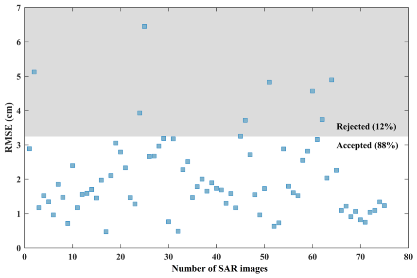
The ZTD at 49 ERA5 grid points (Figure 1e) was utilized for internal quality evaluation. The proposed model estimated ZTD at each grid point for 75 SAR images and calculated the RMSE relative to the original values. SAR images with an RMSE exceeding twice the STD were deemed unsuitable for tropospheric delay correction and discarded. Results showed that 66 images (88%) were accepted, while nine images (12%) were rejected. Consequently, the remaining 66 SAR images were retained as the data source for subsequent research (Figure 7).

Figure 7. Quality evaluation and filter for SAR images based on tropospheric delay.

These 66 SAR images were processed using DS-InSAR to obtain 2145 differential interferograms. Currently, GACOS is the mainstream method for InSAR tropospheric delay correction, serving as a performance benchmark. The STD produced by the proposed model was compared with that of GACOS to assess tropospheric delay reduction. Comparisons included stratified delay-only correction (“only D_stra”) and turbulent delay-only correction (“only D_turb”) to clarify the contribution of each submodel to overall delay mitigation. Table 1 presents the STDs of the original interferograms (2.32 rad), GACOS (1.94 rad), and the proposed model (1.76 rad). GACOS and the proposed model reduced the STD by 16.38% and 24.14%, respectively, compared to the original interferograms, demonstrating the proposed model’s superior performance over GACOS in interferogram tropospheric delay correction. This assessment highlights the relative impact of the stratified and turbulent delay submodels on overall phase correction accuracy. The integration of both components makes the proposed model more robust. These findings support the model’s applicability to diverse InSAR datasets. The STDs for the stratified-delay-only correction and the turbulent-delay-only correction were 1.91 rad and 2.28 rad, respectively, representing reductions of 17.67% and 1.72% compared to the original interferograms. The performance of the stratified-delay-only correction was on par with GACOS. Notably, the STD for the turbulent-delay-only correction was slightly lower than that of the original interferograms, indicating that stratified delays predominantly influenced the original signals. The number of improved interferograms for GACOS, the stratified-delay-only correction, the turbulent-delay-only correction, and the proposed model was 1578, 1519, 1153, and 1790, corresponding to 73.57%, 70.82%, 53.75%, and 83.45% of the dataset, respectively. The proposed model achieved an improvement rate exceeding 80%. However, without correcting the turbulent delay, the improvement rate decreased to 70.82%. Consequently, the turbulent delay cannot be ignored. By addressing both stratified and turbulent delays, the proposed model outperformed the other approaches.

Table 1. Comparison of tropospheric delay correction methods based on 2145 interferograms.

Methods	STD/rad	Imp.Ifgs	Percentage
Original	2.32	\	\
GACOS	1.94 ↓ 16.38%	1578	73.57%
Only Dstra	1.91 ↓ 17.67%	1519	70.82%
Only Dturb	2.28 ↓ 1.72%	1153	53.75%
Proposed model	1.76 ↓ 24.14%	1790	83.45%

↓ represents the percentage reduction compared to the original interferogram.

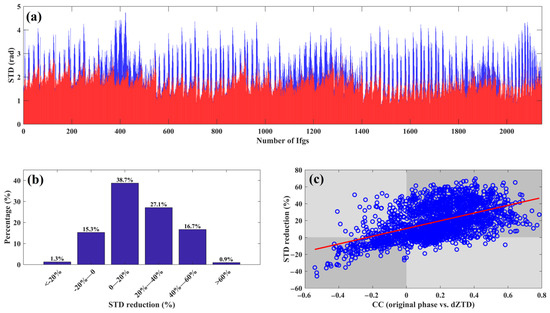
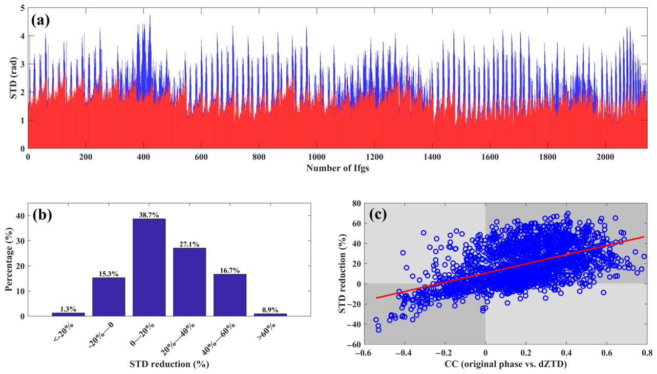
Figure 8a illustrates the STD variations before and after the tropospheric delay correction for all interferograms using the proposed model. Most interferograms exhibited STD reductions from approximately 3 rad to around 2 rad, while some original interferograms reached up to 4 rad, highlighting the substantial influence of tropospheric delays. Figure 8b shows the percentage of STD reduction, with positive and negative values indicating the respective correction directions. The reduction percentages were divided into six intervals: <−20%, −20% to 0%, 0% to 20%, 20% to 40%, 40% to 60%, and >60%. Interferograms within these intervals accounted for 1.3%, 15.3%, 38.7%, 27.1%, 16.7%, and 0.9% of the dataset, respectively. The 0–20% and 20–40% ranges represented 38.7% and 27.1%, collectively comprising over half of all cases. Yu et al. proposed the correlation between the phases and the estimated atmospheric delays as an indicator for the applicability of GACOS [34]. Figure 8c demonstrated the correlation coefficient (CC) between the original phase and differential ZTD (dZTD). Note that dZTD represents the result of the ZTD difference between the two SAR images. After removing terrain and other biases, tropospheric delay became the primary source of interferogram error; thus, a higher original phase-dZTD correlation suggests that dZTDs calculated by the proposed model could better describe the tropospheric delay features in the interferograms. However, there were cases contrary to this trend, such as data points located in two light gray areas.

Figure 8. Evaluation of tropospheric delay correction for the proposed model based on 2145 interferograms. (a) The STD variations before and after the tropospheric delay correction for all interferograms using the proposed model. (b) The percentage of STD reduction. (c) The CC between the original phase and dZTD. Note that the blue columns in (a) represent the STD of the original interferograms; the red columns in (a) represent the STD after the tropospheric delay correction by the proposed model; and the red line in (c) represents the fitting results.

3.3. Evaluation of Correcting Tropospheric Delay for a Single Interferogram

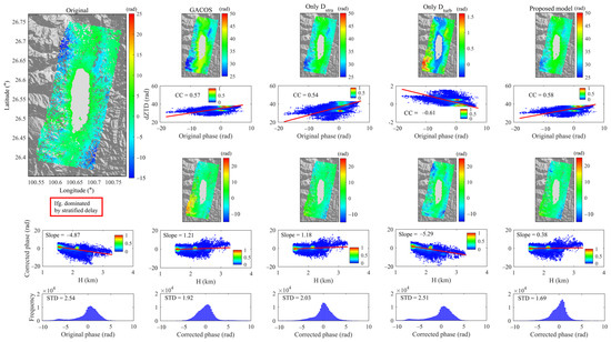
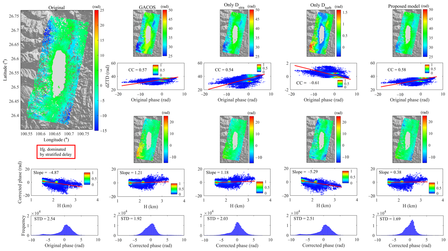
We evaluated various tropospheric correction methods for interferograms using three indicators, such as CC between original phase and dZTD, slope of the linear regression curve between height and corrected phase, and STD. The meaning of CC between the original phase and dZTD has been given above. The indicator of the slope of the linear regression curve between height and corrected phase could reflect the effect of stratified delay correction. STD is an overall indicator. Figure 9 and Figure 10 display interferograms dominated by stratified and turbulent delays, respectively. Tropospheric delays estimated using GACOS and the proposed model were similar, as shown in the first row of Figure 9. In contrast, the turbulent-only correction method produced significantly different tropospheric delays, since turbulent delay is a minor component. The second and fifth rows of Figure 9 illustrate that the STD decreased as the CC between the original phase and dZTD increased, indicating that a higher CC between the original phase and dZTD could better describe the tropospheric delay features in the interferograms. In the third row of Figure 9, corrected interferograms generated by GACOS, the stratified-only method, and the proposed model displayed comparable patterns; however, GACOS results exhibited distinct anomalies in the lower-left corner, likely due to the region’s abrupt undulating terrain. The turbulent-only method yielded interferograms similar to the original, confirming its inability to correct the dominant stratified delay. The fourth and fifth rows of Figure 9 show that a lower slope of the linear regression curve corresponds to a lower STD, signifying that correcting the stratified delay is the key for the interferogram dominated by stratified delay.

Figure 9. Correction example of the interferogram dominated by the stratified delay. Note that the figure in the upper left corner is the original interferogram; the first row is the tropospheric delay estimated by various methods; the second row is the relationship between the dZTD and the original phase; the third row is the interferograms after correcting tropospheric delay; the fourth row is the relationship between height and corrected phase; and the fifth row is the frequency distribution histogram of the original phase and the corrected phase for various methods.

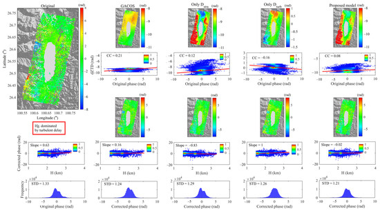
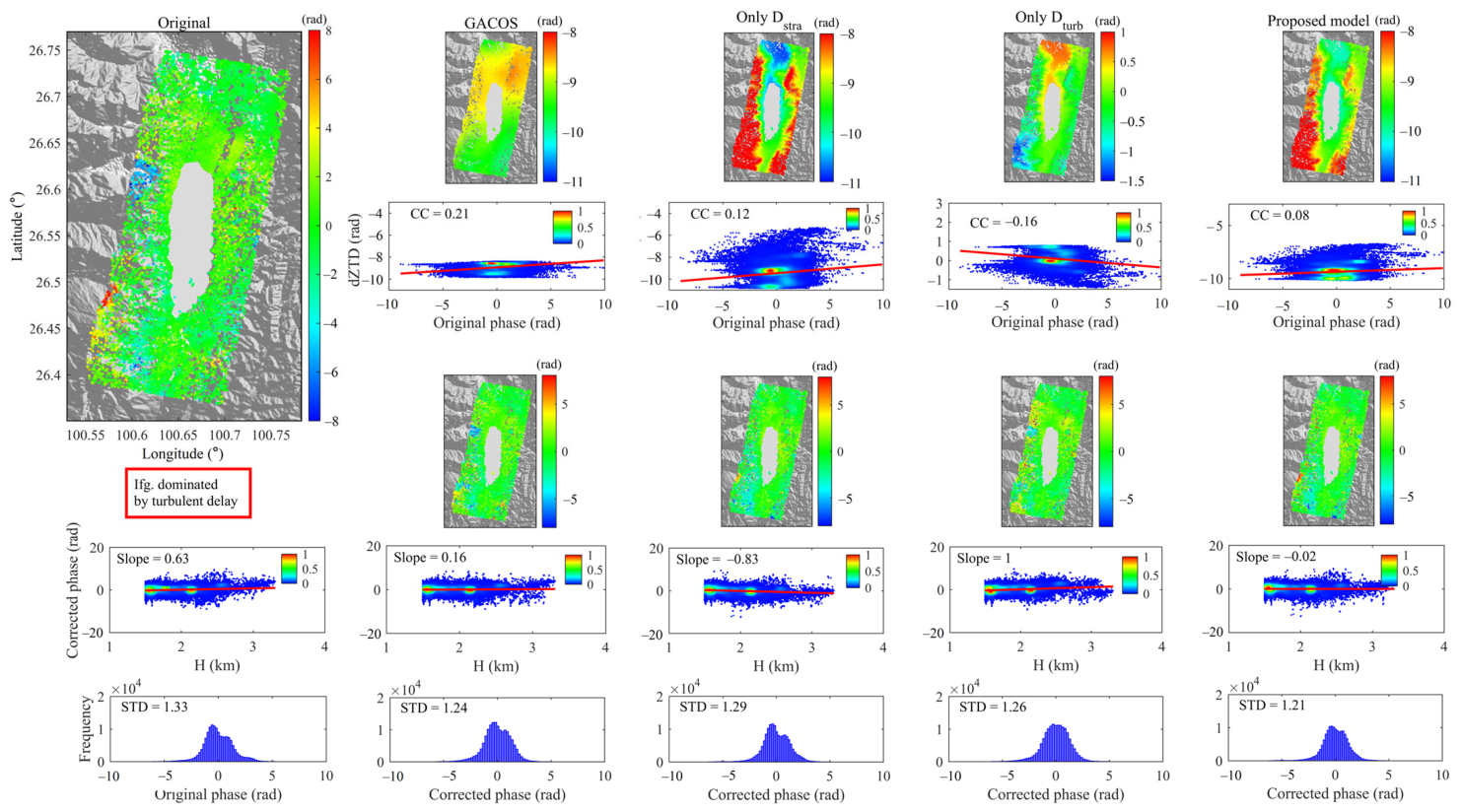
Figure 10. Correction example of the interferogram dominated by turbulent delay.

GACOS yielded a lower STD than the stratified-only correction; however, the stratified-only approach produced a lower slope of the linear regression curve, indicating more effective stratified-delay removal compared to GACOS. Since both stratified and turbulent delays were present in the interferogram, GACOS attained a lower STD than the stratified-only correction by simultaneously compensating for both delays. The CC between dZTD and the original phase for the turbulent-only correction deviated the most from those of the other three methods, signifying an inadequate tropospheric delay correction when stratified delay predominated the interferogram. Furthermore, the slope of the turbulent-only method was almost the same as that of the original interferogram, signifying that the turbulent-only method could not correct the stratified delay. These findings highlight that addressing a single delay component is insufficient for comprehensive STD reduction. In general, a higher CC between the original phase and dZTD or a lower slope of the linear regression curve between height and corrected phase correlates with a lower STD. Thus, the proposed model, by concurrently addressing both stratified and turbulent delays, outperformed methods targeting individual components. After only correcting the stratified delay, the STD was reduced by 0.51 rad compared to the original interferogram, and after further correcting the turbulent delay, the STD was reduced by 0.34 rad again, signifying that establishing the linear relationship between turbulent delay and ZWD to correct the turbulent delay is effective. Therefore, correcting the stratified delay is necessary for the interferogram dominated by the stratified delay. But the correction of the turbulent delay could not be ignored.

As displayed in the first row of Figure 10, tropospheric delay estimates varied significantly across the different methods. In contrast to interferograms dominated by stratified delay, the CC between original phase and dZTD showed no systematic relationship with STD across all four correction methods. CC values were all low for each method because turbulent delay exhibited more stochastic behavior than stratified delay and was susceptible to residual signals. Following tropospheric delay corrections using all four approaches, the interferograms largely preserved the appearance of the original observations (Figure 10, third row). Slope of the linear regression curve between height and corrected phase stayed similar and showed no pattern with STD (Figure 10, fourth row). The highest STD was observed with the stratified-only correction, highlighting its inability to address turbulence. Both GACOS and the proposed model yielded lower STD than the turbulence-only correction, as these two methods simultaneously corrected stratified and turbulent delays, whereas the turbulence-only method addressed only turbulence. The results confirm that stratified delay also exists in interferograms dominated by turbulent delay.

Although the first and second indicators could not draw a conclusion about which method achieves better correction performance, the STD of each method demonstrated that the proposed model achieved the best correction effect. It signifies that ZWD could capture the small-scale variations in turbulent delay. Therefore, by addressing both stratified and turbulent delays, the proposed model delivered superior correction performance, which benefited from the incorporation of time-varying Gaussian coefficients and coupled ZWD. In particular, the proposed model provides a novel and effective way to correct the turbulent delay.

3.4. Overall Evaluation of Correcting Stratified and Turbulent Delays by the Proposed Model

Based on the prior analysis, the proposed model outperformed others in handling interferograms dominated by either stratified or turbulent delays, unlike methods that address only one delay type and thus fail to accommodate all interferograms. To quantitatively evaluate the systematic bias and stability of different correction models for correcting stratified delay, we propose utilizing the geometric attributes of the quadratic fitting curves between the STD reduction and the original phase-elevation CC. Specifically, a parabolic symmetry axis closer to zero serves as a critical indicator of reduced systematic error, whereas a parabola vertex closer to zero reflects the stability of the correction. The same approach is utilized for the quantitative evaluation of turbulent delay correction.

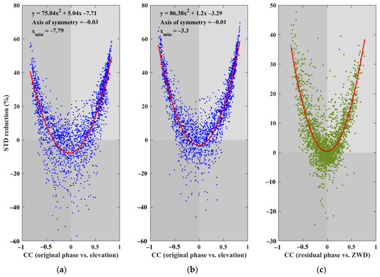
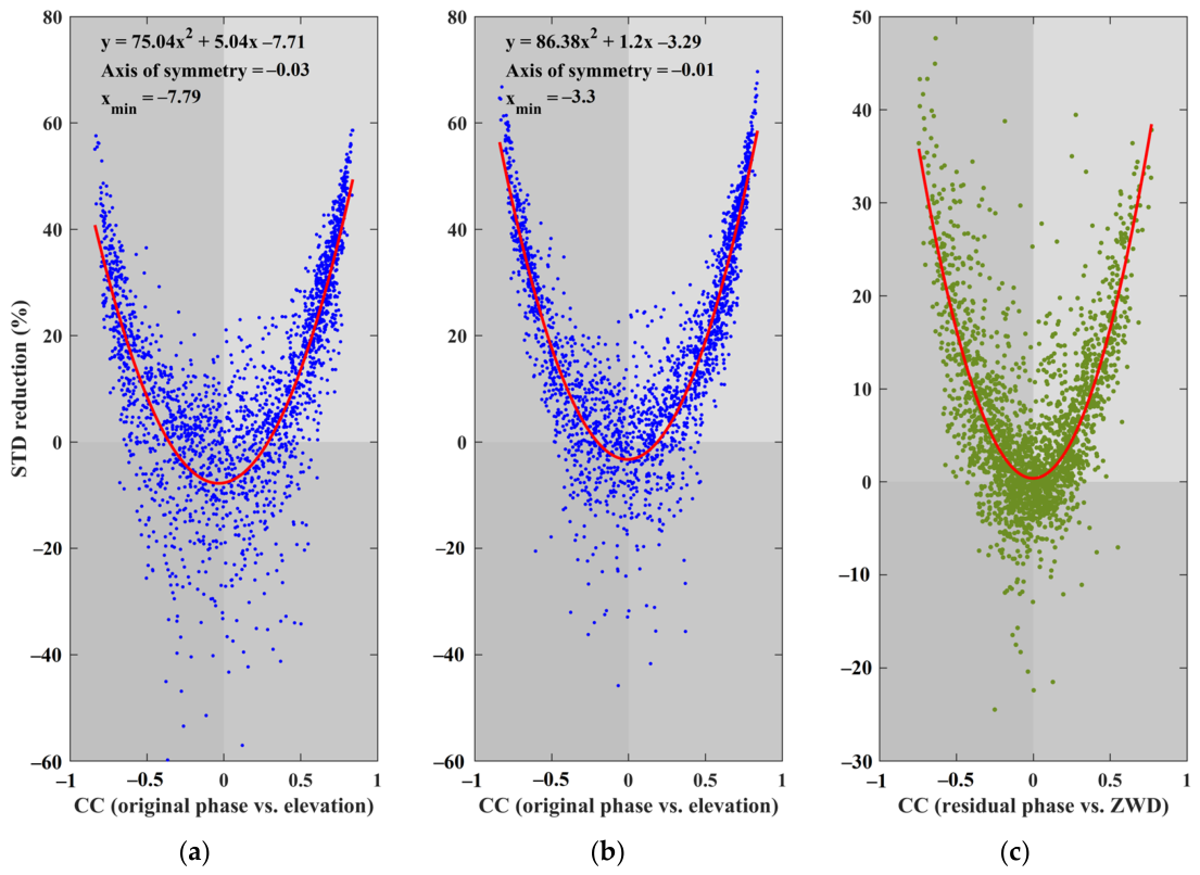
We further assessed the ability of the model to correct both stratified and turbulent delays for all interferograms. Figure 11a,b illustrate the relationship between STD reduction and original phase-elevation CC for GACOS and the proposed model, respectively. The upward-opening red quadratic fitting curves demonstrate that higher absolute CC values correspond to greater STD reductions, indicating more effective stratified delay corrections. The symmetry axes for GACOS (−0.03) and the proposed model (−0.01) exhibit that the axis of the proposed model is closer to zero. Additionally, the minimum STD reductions for GACOS (−7.79) and the proposed model (−3.3) indicate that the proposed model achieves values nearer to zero. These two parameters are essential indicators of correction bias and stability. A symmetry axis closer to zero signifies reduced systematic error, whereas a less negative parabola vertex indicates improved stability.

Figure 11. (a) Performance of correcting stratified delay by GACOS. (b) Performance of correcting stratified delay by the proposed model. (c) Performance of correcting the turbulent delay by the proposed model. Note that the red lines represent the fitting results.

This analysis confirmed a stronger correlation between STD reduction and CC, resulting in more stable stratified delay correction by the proposed model. Figure 11c displays the turbulent delay correction performance exclusively for the proposed model, as GACOS is incapable of providing only turbulent delay. It was essential to correct the stratified delay in the interferograms before evaluating the turbulent delay correction. We established the relationship between the residual phase and ZWD to address turbulent delay. The results showed that the red fitting curve of STD reduction versus the CC between residual phase and ZWD formed an upward-opening parabola. This pattern indicated that larger absolute CC values led to greater STD reductions, signifying more effective turbulent delay correction. However, many interferograms exhibited low CCs, causing suboptimal corrections. This outcome likely resulted from highly random, turbulent delays that ZWD could not capture.

3.5. Evaluation of Deformation Velocities and Time Series

Previous analyses focused solely on interferograms, whereas InSAR aims to derive deformation time series and rates. We integrated the proposed model into StaMPS and computed each SAR image’s tropospheric delay, subtracted these delays from the unwrapped interferograms, and reran the unwrapping. Finally, we obtained surface deformation velocities and time series for the Chenghai Lake region in Northwest Yunnan.

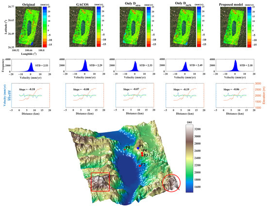
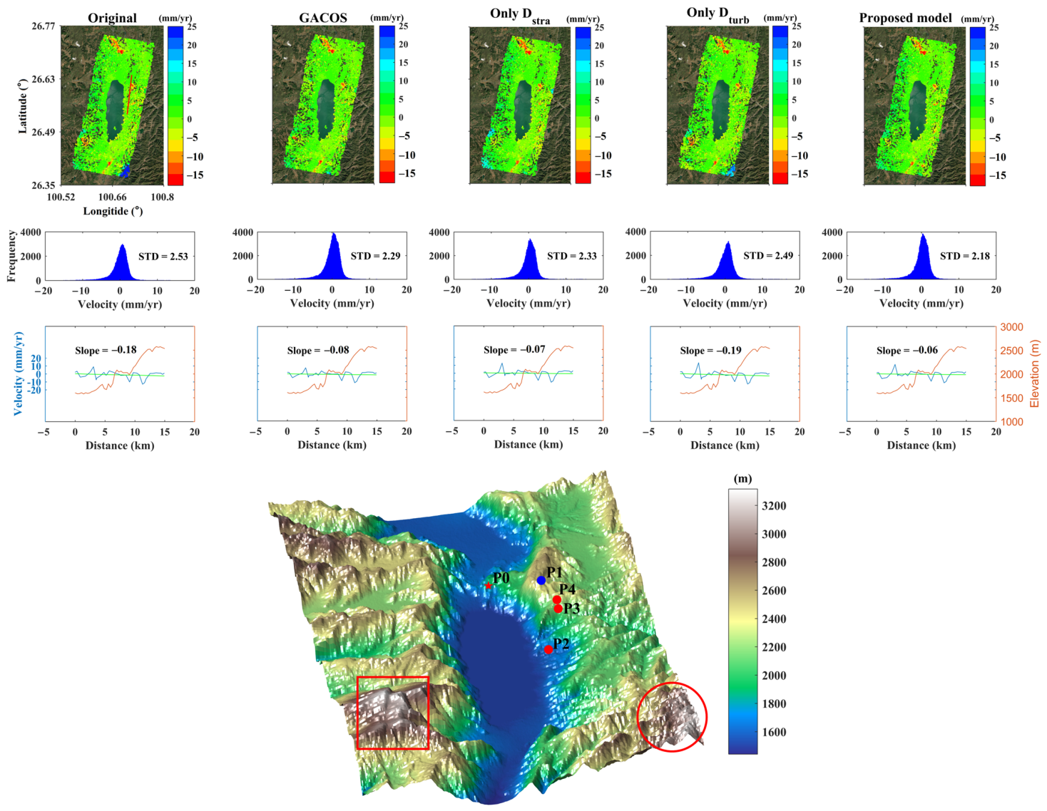
Figure 12 (first row) illustrates the original deformation velocity alongside those derived from four distinct tropospheric delay correction methods. Each method demonstrated varying degrees of improvement compared to the uncorrected data, highlighting their differing capacities to mitigate tropospheric artifacts. These enhancements varied in both spatial distribution and magnitude across the study area. The regions enclosed by the red box and circle exhibit significant undulating terrain and experienced substantial stratified delay. Notably, the proposed method achieved the most effective reduction in stratified delay among all four approaches. The stratified-only correction yielded comparable results, whereas GACOS failed to eliminate the stratified delay, leaving residual stratification within the interferogram, particularly inside the red box. In contrast, the turbulent-only correction was the least effective, closely resembling the uncorrected results and confirming that stratified delay dominated the error budget, making turbulence correction alone insufficient. Figure 12 (second row) illustrates the deformation velocity STD and its histogram distribution corresponding to Figure 12 (first row). The proposed method achieved the lowest STD among all four approaches, signifying that the proposed method greatly weakened the oscillation of deformation velocity caused by tropospheric delay.

Figure 12. Evaluation of deformation velocity. The first row is the deformation velocity of the original and the four methods. The second row displays the deformation velocity STD and corresponding histograms. The third row is the deformation velocity on the profile line. The fourth row is the DEM. Note that the red straight line represents the profile line; the red box and circle represent the regions with considerable undulating terrain; the orange lines in the third row represent the elevation; the blue lines in the third row represent the deformation velocity; and the green lines in the third row represent the fitting result of the deformation velocity.

To examine the relationship between topography and deformation before and after tropospheric delay compensation, a profile line approximately 15 km long was extracted (Figure 12, third row). This profile spans an elevation variation of approximately 1 km and serves as the basis for analyzing the dependence between terrain features and deformation velocities [55]. Although visual inspection did not show significant differences among the five results, all methods except the turbulent-delay-only correction partially alleviated the dependence between deformation velocity and terrain. The slope of the green fitting line served as the evaluation metric. The turbulent-delay-only correction failed to reduce the impact of undulating terrain because it did not address stratified delay. In contrast, the proposed model achieved a slightly lower slope than both GACOS and the stratified-delay-only correction, demonstrating better mitigation of stratified delay. Consequently, the proposed model outperformed alternative methods in managing terrain-induced fluctuations.

GNSS-derived displacement was used as the reference to assess deformation time-series accuracy for both GACOS and the proposed model. Prior to evaluation, 3D GNSS displacements were projected onto the Sentinel-1A LOS.

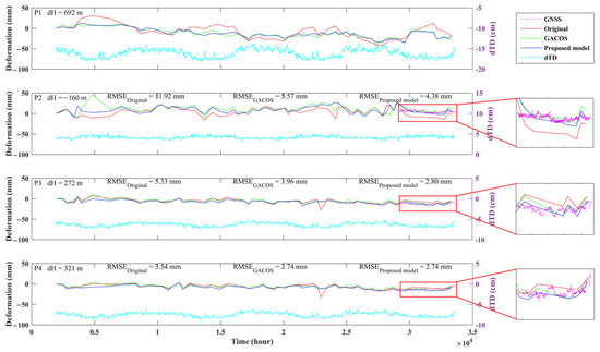
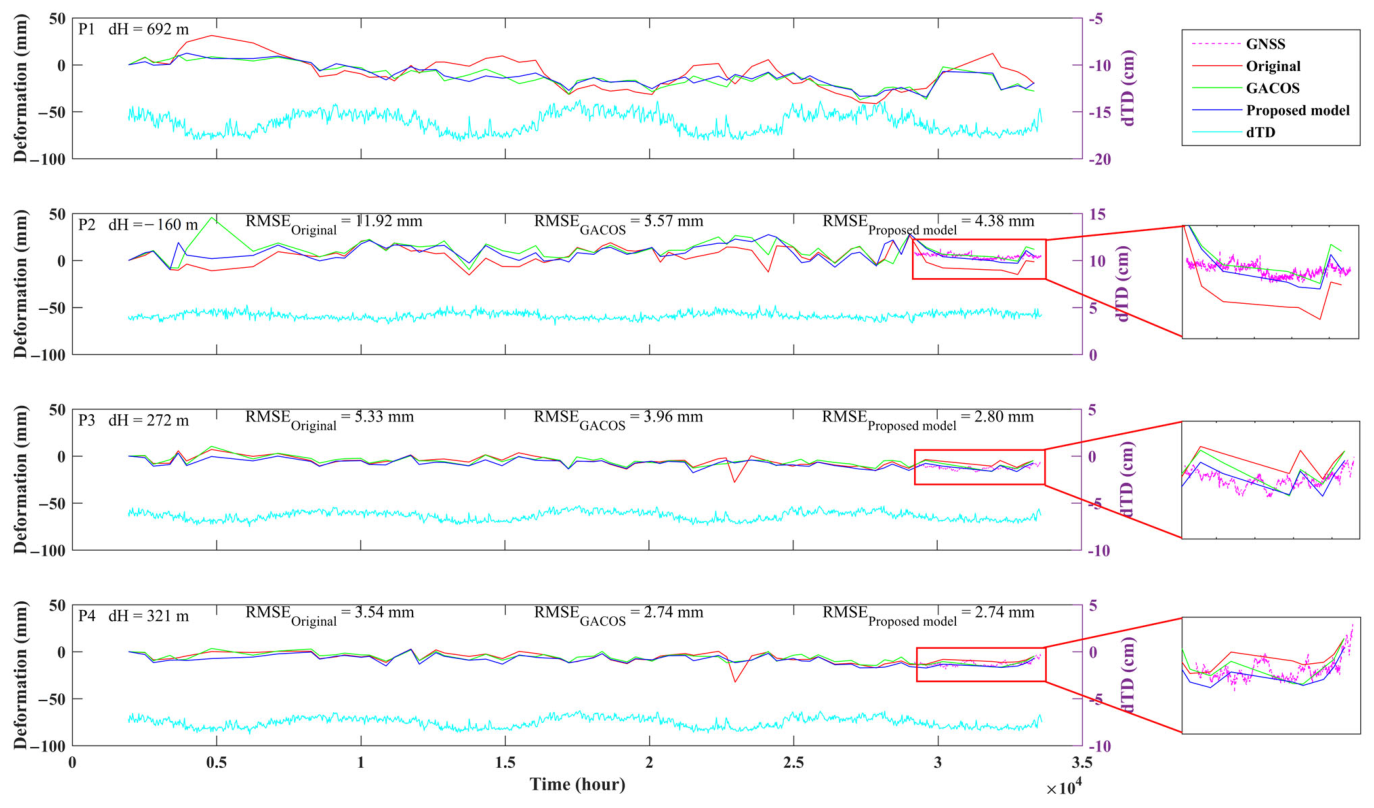
In Figure 13, we assess the deformation time series at points P1–P4, with P0 serving as the unwrapping reference. Their locations are shown in the DEM in the third row of Figure 12, illustrating the spatial distribution of all five monitoring sites. In Figure 13, dH represents the differential height between each measurement point and P0. The dZTD amplitude at P1 was the greatest among all points, underscoring the relationship between dH magnitude and seasonal tropospheric delay. Consequently, the uncorrected time series exhibited seasonal variations, indicating an influence from tropospheric delay. This seasonal impact was mitigated following tropospheric delay correction using either GACOS or the proposed model. The dH values for P2, P3, and P4 were −160 m, 272 m, and 321 m, respectively. As absolute dH increased, the seasonal oscillation of dZTD became more pronounced, and the unadjusted deformation time series was increasingly affected by seasonal variation.

Figure 13. Evaluation of deformation time series using GNSS data. Note that dH represents the differential height between each measurement point and P0.

We compared the proposed model with GACOS using GNSS-derived displacement time series at P2–P4. Both corrected series more closely matched the true deformation than the uncorrected results; visually, the proposed model aligned more closely with the reference observations than GACOS. The RMSE, used as an accuracy metric, was computed against the reference displacement data. At processing points P2, P3, and P4, the RMSE values for the original results, GACOS, and the proposed model were 11.92, 5.57, and 4.38 mm; 5.33, 3.96, and 2.80 mm; and 3.54, 2.74, and 2.74 mm, respectively. These quantitative findings demonstrate that the proposed model achieved a lower RMSE than GACOS at P2 and P3, with reductions of 21.4% and 29.3%, respectively. At P4, both methods yielded identical RMSE values. Overall, integrating the proposed model into StaMPS enhanced the accuracy of deformation time series compared to GACOS. This result benefits from the stratified delay model that accounts for time-varing Gaussion coefficients and the turbulent delay model that couples ZWD.

4. Discussion

By allowing Gaussian coefficients to vary temporally, the stratified delay model improved ZTD vertical interpolation accuracy relative to the assumption of constant coefficients.

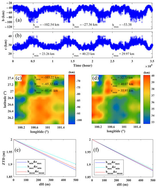
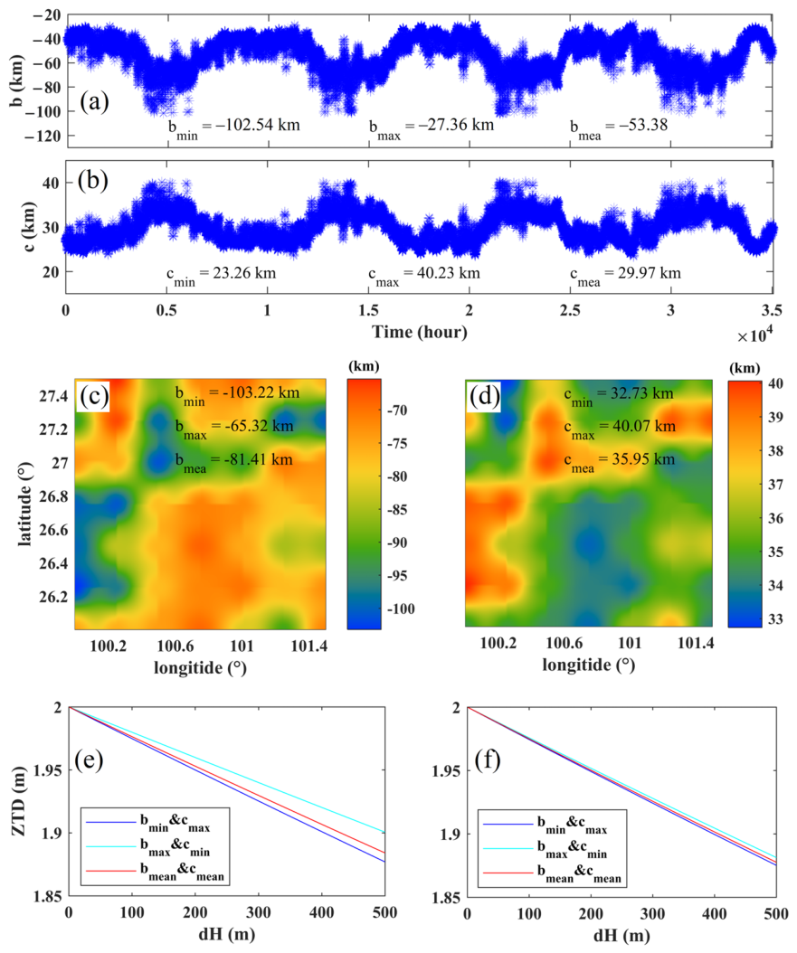
Figure 14a,b depict the time series of Gaussian coefficients b and c at the grid point (26.5° N, 100.75° E) from 2019 to 2022. For coefficient b, the minimum, maximum, and mean values were −102.54, −27.36, and −53.38 km, respectively; for coefficient c, they were 23.26, 40.23, and 29.97 km. These coefficients exhibited seasonal periodicity. The impact of assuming constant Gaussian coefficients on ZTD vertical interpolation was previously discussed. The Gaussian coefficient b achieved its lowest value in summer, whereas coefficient c attained its highest. For clarity, the combination with minimum b and maximum c in time or space is designated as $b_{min}\&c_{max}$, the combination with maximum b and minimum c as $b_{max}\&c_{min}$, and the combination with mean b and mean c as $b_{mean}\&c_{mean}$. Figure 14e illustrates the vertical interpolation of ZTD using $b_{min}\&c_{max}$, $b_{max}\&c_{min}$, and $b_{mean}\&c_{mean}$ over time, utilizing Equation (6). When the stratified delay model employed $b_{min}\&c_{max}$ temporally, the deviation between $b_{min}\&c_{max}$ and $b_{max}\&c_{min}$ was 1.65 cm at dH = 500 m, and between $b_{mean}\&c_{mean}$ and $b_{max}\&c_{min}$ was −0.71 cm. These deviations were unacceptable.

Figure 14. Temporal and spatial variation range of Gaussian coefficients and its influence on ZTD vertical interpolation. (a) Time series of Gaussian coefficient b. (b) Time series of Gaussian coefficient c. (c) The spatial distribution of Gaussian coefficient b. (d) The spatial distribution of Gaussian coefficient c. (e) The ZTD vertical interpolation with different combinations in time. (f) The ZTD vertical interpolation with different combinations in space.

Figure 14c,d display the spatial distribution of b and c at 23:00 on 20 July 2019. The minimum, maximum, and mean values of b were −103.22, −65.32, and −81.41 km, respectively; for c, they were 32.73, 40.07, and 35.95 km. The spatial variation in the Gaussian coefficients was pronounced. Figure 14f presents the vertical interpolation of ZTD using the three combinations in space. The stratified delay model utilized the spatial combination of $b_{mean}\&c_{mean}$, and the spatial deviation between $b_{min}\&c_{max}$ and $b_{mean}\&c_{mean}$ was 0.37 cm, and between $b_{max}\&c_{min}$ and $b_{mean}\&c_{mean}$ was −0.24 cm for dH = 500 m. These deviations were smaller than those observed with the temporal combination. Specifically, these results indicate that spatial variability introduces less error than temporal variability under the evaluated conditions. Therefore, incorporating time-varying Gaussian coefficients was essential in developing the stratified delay model. Additionally, Gaussian coefficients were derived at DEM points with a 30 m resolution to capture spatial variations.

Three scenarios based on mean Gaussian coefficients—temporal (Plan T), spatial (Plan S), and spatiotemporal (Plan TS)—were created to evaluate their impact on InSAR measurements. For ease of reference, these scenarios are referred to as Plan T, Plan S, and Plan TS, respectively. Furthermore, the coupling-ZWD method was used to estimate turbulent delay and compared with the conventional filtering method (Plan F). Importantly, the proposed stratified delay model was applied to correct the stratified delay prior to filtering.

Table 2 lists the phase STD and deformation RMSE for the proposed model and the four plans. The STD for Plans T, S, and TS were 1.79, 1.78, and 1.80 rad, respectively, representing increases of 1.70%, 1.14%, and 2.27% compared to the STD of the proposed model of 1.79 rad. Plan TS exhibited the greatest increase in STD, whereas the STD of Plan T increased more than that of Plan S, indicating that temporal errors from mean Gaussian coefficients outweighed spatial errors. Compared to the proposed model, deformation RMSE increased by 3.13%, 2.19%, and 3.76% for Plans T, S, and TS, respectively. The STD and RMSE of Plan F increased by 7.39% and 15.36%, respectively, relative to the proposed model, demonstrating that using ZWD to capture turbulent delay variations outperformed the filtering method. The limitations of the filtering method potentially originated from its assumption of spatial atmospheric correlation and temporal randomness; seasonal variations in atmospheric parameters, especially water vapor, violated this assumption.

Table 2. Statistics of phase STD and deformation RMSES for various tropospheric delay correction models.

Methods	STD/rad	Defor RMSE/mm
Proposed model	1.76	3.19
Plan T	1.79 ↑ 1.70%	3.29 ↑ 3.13%
Plan S	1.78 ↑ 1.14%	3.26 ↑ 2.19%
Plan TS	1.80 ↑ 2.27%	3.31 ↑ 3.76%
Plan F	1.89 ↑ 7.39%	3.68 ↑ 15.36%

↑ represents the the percentage increase compared to the proposed model.

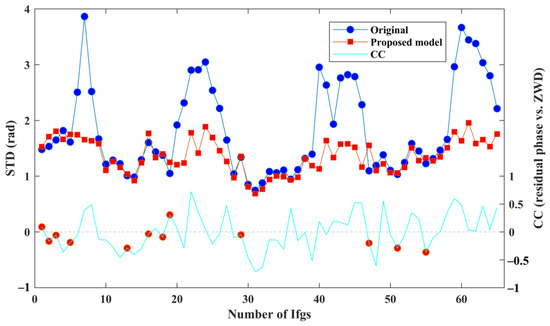
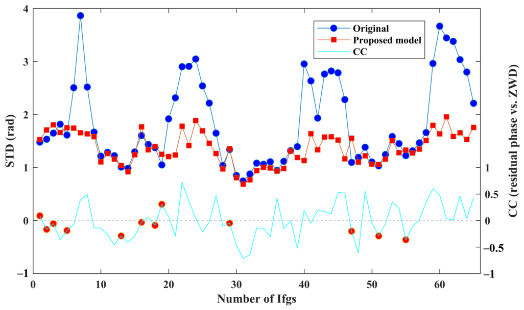
After the tropospheric delay correction, not all interferograms improved; some STDs increased. Figure 15 displays the phase STD and the CC between turbulent delay and ZWD for 65 interferograms, using the SAR image from 10 January 2011, as the master image, thereby investigating the causes of negative corrections. Twelve interferograms (18.46%) were categorized into the negative correction group, with a maximum deviation of 0.47 rad and an average deviation of 0.13 rad. This effect on the final deformation was minimal and negligible. In the negative correction group, the CC was nearly zero, with a mean absolute CC of 0.18, falling below the overall interferogram mean of 0.26. This indicates that ZWD in this group fails to reflect turbulent delay, resulting in a suboptimal turbulent correction. This shortcoming is potentially because of the significant randomness in turbulent delays, leading to incomplete or inaccurate estimations of turbulent delays.

Figure 15. Phase STD and CC between the turbulent delay and ZWD for 65 interferograms. Note that the red dots represent the CC of the negative correction group.

5. Conclusions

This study introduces a model that integrates ERA5 and GNSS data into StaMPS to correct stratified and turbulent delays, thereby effectively mitigating stratified and turbulent InSAR delays in alpine canyon regions. The stratified correction utilizes time-varying Gaussian coefficients to address seasonal delay oscillations. For turbulent correction, a linear relationship between turbulent delay and ZWD is established to capture small-scale tropospheric delay variations. The proposed model successfully captures both seasonal and diurnal delay variations. The STD of its phase decreased by 9.28% compared to GACOS, and it increases the number of improved interferograms by 13.43% relative to GACOS. In two interferogram examples dominated by stratified and turbulent delays, the proposed model outperformed GACOS in correcting tropospheric delays. Methods that exclusively address either stratified or turbulent delays are not universally applicable to all interferogram types. Deformation velocities obtained from the proposed model exhibited reduced terrain dependency. The deformation RMSE values were 4.09 mm for GACOS and 3.31 mm for the proposed model. Both methods mitigated seasonal oscillations in deformation time series caused by tropospheric delays; quantitative analysis shows that the proposed model achieved 19.07% higher accuracy than GACOS. Furthermore, we evaluated the necessity of incorporating time-varying Gaussian coefficients and the role of coupled ZWD in turbulent delay correction. Using a temporal constant average Gaussian coefficient increased the phase STD and deformation RMSE by 1.70% and 3.13%, respectively, compared to the proposed model, thereby confirming the need for time-varying coefficients. Conventional filtering did not outperform the proposed model in addressing turbulent delays. Negative corrections in interferograms were associated with random turbulent delay intensities.

The proposed model provides two distinct advantages over GACOS. First, it incorporates a time-varying vertical variation factor into tropospheric delay estimation. Second, it employs a coupling strategy that integrates ZWD estimates into delay-correction procedures to reduce turbulent delay. Nonetheless, the model has certain limitations. For example, although it captures the diurnal ZTD trend, it exhibits suboptimal fitting quality. Moreover, the effectiveness of turbulent-delay correction depends on the stochastic properties of turbulence; significant randomness prevents ZWD from accurately representing turbulent-delay variations, thereby constraining overall performance. Consequently, future research will focus on optimizing the turbulent-delay model to enhance fitting accuracy and robustness under varying atmospheric conditions.

References

- Abidin, H.; Andreas, H.; Gamal, M.; Wirakusumah, A.; Darmawan, D.; Deguchi, T.; Maruyama, Y. Land Subsidence Characteristics of the Bandung Basin, Indonesia, as Estimated from GPS and InSAR. J. Appl. Geod. 2008, 2, 167–177. [Google Scholar] [CrossRef]
- Xu, B.; Li, Z.W.; Feng, G.C.; Zhang, Z.Y.; Wang, Q.J.; Hu, J.; Chen, X.G. Continent-Wide 2-D Co-Seismic Deformation of the 2015 Mw 8.3 Illapel, Chile Earthquake Derived from Sentinel-1A Data: Correction of Azimuth Co-Registration Error. Remote Sens. 2016, 8, 376. [Google Scholar] [CrossRef]
- Sigmundsson, F.; Hreinsdóttir, S.; Hooper, A.; Arnadóttir, T.; Pedersen, R.; Roberts, M.J.; Óskarsson, N.; Auriac, A.; Decriem, J.; Einarsson, P. Intrusion Triggering of the 2010 Eyjafjallajökull Explosive Eruption. Nature 2010, 468, 426–430. [Google Scholar] [CrossRef] [PubMed]
- Morales Rivera, A.M.; Amelung, F.; Mothes, P.; Hong, S.-H.; Nocquet, J.-M.; Jarrin, P. Ground Deformation before the 2015 Eruptions of Cotopaxi Volcano Detected by InSAR. Geophys. Res. Lett. 2017, 44, 6607–6615. [Google Scholar] [CrossRef]
- Yang, Z.; Li, Z.; Zhu, J.; Yi, H.; Hu, J.; Feng, G. Deriving Dynamic Subsidence of Coal Mining Areas Using InSAR and Logistic Model. Remote Sens. 2017, 9, 125. [Google Scholar] [CrossRef]
- Galetzka, J.; Melgar, D.; Genrich, J.F.; Geng, J.; Owen, S.; Lindsey, E.O.; Xu, X.; Bock, Y.; Avouac, J.-P.; Adhikari, L.B. Slip Pulse and Resonance of the Kathmandu Basin during the 2015 Gorkha Earthquake, Nepal. Science 2015, 349, 1091–1095. [Google Scholar] [CrossRef] [PubMed]
- Feng, G.; Jonsson, S.; Klinger, Y. Which Fault Segments Ruptured in the 2008 Wenchuan Earthquake and Which Did Not? New Evidence from Near-fault 3D Surface Displacements Derived from SAR Image Offsets. Bull. Seismol. Soc. Am. 2017, 107, 1185–1200. [Google Scholar] [CrossRef]
- Watt, J.; Ponce, D.; Parsons, T.; Hart, P. Missing Link between the Hayward and Rodgers Creek Faults. Sci. Adv. 2016, 2, e1601441. [Google Scholar] [CrossRef] [PubMed]
- Hooper, A.; Bekaert, D.; Spaans, K.; Arıkan, M. Recent Advances in SAR Interferometry Time Series Analysis for Measuring Crustal Deformation. Tectonophysics 2012, 514, 1–13. [Google Scholar] [CrossRef]
- Bekaert, D.P.S.; Walters, R.J.; Wright, T.J.; Hooper, A.J.; Parker, D.J. Statistical Comparison of InSAR Tropospheric Correction Techniques. Remote Sens. Environ. 2015, 170, 40–47. [Google Scholar] [CrossRef]
- Wang, S.; Lu, Z.; Wang, B.; Niu, Y.; Song, C.; Li, X.; Ma, Z.F.; Xu, C.J. A Phase-Based InSAR Tropospheric Correction Method for Interseismic Deformation Based on Short-Period Interferograms. IEEE Trans. Geosci. Remote Sens. 2023, 61, 5212318. [Google Scholar] [CrossRef]
- Ferretti, A.; Prati, C.; Rocca, F. Permanent Scatterers in SAR Interferometry. IEEE Trans. Geosci. Remote Sens. 2001, 39, 8–20. [Google Scholar] [CrossRef]
- Berardino, P.; Fornaro, G.; Lanari, R.; Sansosti, E. A New Algorithm for Surface Deformation Monitoring Based on Small Baseline Differential SAR Interferograms. IEEE Trans. Geosci. Remote Sens. 2002, 40, 2375–2383. [Google Scholar] [CrossRef]
- Hooper, A.; Zebker, H.; Segall, P.; Kampes, B. A New Method for Measuring Deformation on Volcanoes and Other Natural Terrains Using InSAR Persistent Scatterers. Geophys. Res. Lett. 2004, 31, L23611. [Google Scholar] [CrossRef]
- Ferretti, A.; Fumagalli, A.; Novali, F.; Prati, C.; Rocca, F.; Rucci, A. A New Algorithm for Processing Interferometric Data-Stacks: SqueeSAR. IEEE Trans. Geosci. Remote Sens. 2011, 49, 3460–3470. [Google Scholar] [CrossRef]
- He, X.; Li, Z.; Mu, M.; Duan, M.; Wei, J.; Cao, Y. Advanced Tropospheric Delay Mitigation Method Using InSAR-Based Iterative Decomposition by Considering the Statistical Characteristics of Atmospheric Turbulence. IEEE Trans. Geosci. Remote Sens. 2024, 62, 5204710. [Google Scholar] [CrossRef]
- Raucoules, D.; De Michele, M. Assessing Ionospheric Influence on L-Band SAR Data: Implications on Coseismic Displacement Measurements of the 2008 Sichuan Earthquake. IEEE Geosci. Rem. Sens. Lett. 2010, 7, 286–290. [Google Scholar] [CrossRef]
- Fattahi, H.; Simons, M.; Agram, P. InSAR Time-Series Estimation of the Ionospheric Phase Delay: An Extension of the Split Range-Spectrum Technique. IEEE Trans. Geosci. Remote Sens. 2017, 55, 5984–5996. [Google Scholar] [CrossRef]
- Wang, X.; Zeng, Q.; Jiao, J.; Hao, Z. Evaluation of Weather Research and Forecast (WRF) Microphysics Schemes in Simulating Zenith Total Delay for InSAR Atmospheric Correction. Int. J. Remote Sens. 2021, 42, 3456–3473. [Google Scholar] [CrossRef]
- Dong, J.; Zhang, L.; Liao, M.; Gong, J. Improved Correction of Seasonal Tropospheric Delay in InSAR Observations for Landslide Deformation Monitoring. Remote Sens. Environ. 2019, 233, 111370. [Google Scholar] [CrossRef]
- Zhao, Z.; Wu, Z.; Zheng, Y.; Ma, P. Recurrent Neural Networks for Atmospheric Noise Removal from InSAR Time Series with Missing Values. ISPRS J. Photogramm. Remote Sens. 2021, 180, 227–237. [Google Scholar] [CrossRef]
- Jung, J.; Kim, D.; Park, S. Correction of Atmospheric Phase Screen in Time Series InSAR Using WRF Model for Monitoring Volcanic Activities. IEEE Trans. Geosci. Remote Sens. 2013, 52, 2678–2689. [Google Scholar] [CrossRef]
- Xiao, R.Y.; Yu, C.; Li, Z.H.; He, X.F. Statistical Assessment Metrics for InSAR Atmospheric Correction: Applications to Generic Atmospheric Correction Online Service for InSAR (GACOS) in Eastern China. Int. J. Appl. Earth Obs. 2021, 96, 102289. [Google Scholar] [CrossRef]
- Emardson, T.R.; Simons, M.; Webb, F.H. Neutral Atmospheric Delay in Interferometric Synthetic Aperture Radar Applications: Statistical Description and Mitigation. J. Geophys. Res. Solid Earth 2003, 108, 2231. [Google Scholar] [CrossRef]
- Wang, Y.; Dong, J.; Zhang, L.; Zhang, L.; Deng, S.; Zhang, G.; Liao, M.; Gong, J. Refined InSAR Tropospheric Delay Correction for Wide-Area Landslide Identification and Monitoring. Remote Sens. Environ. 2022, 275, 113013. [Google Scholar] [CrossRef]
- Walters, R.J.; Elliott, J.R.; Li, Z.; Parsons, B. Rapid Strain Accumulation on the Ashkabad Fault (Turkmenistan) from Atmosphere-corrected InSAR. J. Geophys. Res. Solid Earth 2013, 118, 3674–3690. [Google Scholar] [CrossRef]
- Fattahi, H.; Amelung, F. InSAR Bias and Uncertainty Due to the Systematic and Stochastic Tropospheric Delay. J. Geophys. Res. Solid Earth 2015, 120, 8758–8773. [Google Scholar] [CrossRef]
- Tang, W.; Liao, M.; Yuan, P. Atmospheric Correction in Time-Series SAR Interferometry for Land Surface Deformation Mapping–A Case Study of Taiyuan, China. Adv. Space Res. 2016, 58, 310–325. [Google Scholar] [CrossRef]
- Darvishi, M.; Cuozzo, G.; Bruzzone, L.; Nilfouroushan, F. Performance Evaluation of Phase and Weather-Based Models in Atmospheric Correction with Sentinel-1data: Corvara Landslide in the Alps. IEEE J. Sel. Top. Appl. Earth Obs. Remote Sens. 2020, 13, 1332–1346. [Google Scholar] [CrossRef]
- Jolivet, R.; Agram, P.S.; Lin, N.Y.; Simons, M.; Doin, M.-P.; Peltzer, G.; Li, Z. Improving InSAR Geodesy Using Global Atmospheric Models. J. Geophys. Res. 2014, 119, 2324–2341. [Google Scholar] [CrossRef]
- Bekaert, D.P.S.; Hooper, A.; Wright, T.J. A Spatially Variable Power Law Tropospheric Correction Technique for InSAR Data. J. Geophys. Res. 2015, 120, 1345–1356. [Google Scholar] [CrossRef]
- Elliott, J.R.; Biggs, J.; Parsons, B.; Wright, T.J. InSAR Slip Rate Determination on the Altyn Tagh Fault, Northern Tibet, in the Presence of Topographically Correlated Atmospheric Delays. Geophys. Res. Lett. 2008, 35, L12309. [Google Scholar] [CrossRef]
- Fattahi, H.; Agram, P.; Simons, M. A Network-Based Enhanced Spectral Diversity Approach for TOPS Time-Series Analysis. IEEE Trans. Geosci. Remote Sens. 2017, 55, 777–786. [Google Scholar] [CrossRef]
- Yu, C.; Li, Z.; Penna, N.T.; Crippa, P. Generic Atmospheric Correction Model for Interferometric Synthetic Aperture Radar Observations. J. Geophys. Res. 2018, 123, 9202–9222. [Google Scholar] [CrossRef]
- Yu, C.; Penna, N.T.; Li, Z. Generation of Real-time Mode High-resolution Water Vapor Fields from GPS Observations. J. Geophys. Res. 2017, 122, 2008–2025. [Google Scholar] [CrossRef]
- Yu, C.; Li, Z.; Penna, N.T. Interferometric Synthetic Aperture Radar Atmospheric Correction Using a GPS-Based Iterative Tropospheric Decomposition Model. Remote Sens. Environ. 2018, 204, 109–121. [Google Scholar] [CrossRef]
- Yu, C.; Li, Z.; Penna, N.T. Triggered Afterslip on the Southern Hikurangi Subduction Interface Following the 2016 Kaikōura Earthquake from InSAR Time Series with Atmospheric Corrections. Remote Sens. Environ. 2020, 251, 112097. [Google Scholar] [CrossRef]
- Zhang, X.; Li, Z.; Liu, Z. Reduction of Atmospheric Effects on InSAR Observations through Incorporation of GACOS and PCA into Small Baseline Subset InSAR. IEEE Trans. Geosci. Remote Sens. 2023, 61, 5209115. [Google Scholar] [CrossRef]
- Liang, H.; Zhang, L.; Lu, Z.; Li, X. Correction of Spatially Varying Stratified Atmospheric Delays in Multitemporal InSAR. Remote Sens. Environ. 2023, 285, 113382. [Google Scholar] [CrossRef]
- Murray, K.D.; Bekaert, D.P.; Lohman, R.B. Tropospheric Corrections for InSAR: Statistical Assessments and Applications to the Central United States and Mexico. Remote Sens. Environ. 2019, 232, 111326. [Google Scholar] [CrossRef]
- Wang, X.; Zhu, G.; Huang, L.; Wang, H.; Yang, Y.; Li, J.; Huang, L.; Zhou, L.; Liu, L. Development of a ZTD Vertical Profile Model Considering the Spatiotemporal Variation of Height Scale Factor with Different Reanalysis Products in China. Atmosphere 2022, 13, 1469. [Google Scholar] [CrossRef]
- Li, H.; Zhu, G.; Kang, Q.; Huang, L.; Wang, H. A Global Zenith Tropospheric Delay Model with ERA5 and GNSS-Based ZTD Difference Correction. GPS Solut. 2023, 27, 154. [Google Scholar] [CrossRef]
- Guo, S.; Zuo, X.; Zhang, J.; Yang, X.; Huang, C.; Yue, X. Mountain Landslide Monitoring Using a DS-InSAR Method Incorporating a Spatio-Temporal Atmospheric Phase Screen Correction Model. Remote Sens. 2024, 16, 4228. [Google Scholar] [CrossRef]
- Guo, S.; Zuo, X.; Wu, W.; Yang, X.; Zhang, J.; Li, Y.F.; Huang, C.; Bu, J.; Zhu, S. Mitigation of Tropospheric Delay Induced Errors in TS-InSAR Ground Deformation Monitoring. Int. J. Digit. Earth 2024, 17, 2316107. [Google Scholar] [CrossRef]
- Cao, Y.; Jonsson, S.; Li, Z. Advanced InSAR Tropospheric Corrections from Global Atmospheric Models That Incorporate Spatial Stochastic Properties of the Troposphere. J. Geophys. Res. Solid Earth 2021, 126, e2020JB020952. [Google Scholar] [CrossRef]
- Li, Z.; Cao, Y.; Wei, J.; Duan, M.; Wu, L.; Hou, J.; Zhu, J. Time-Series InSAR Ground Deformation Monitoring: Atmospheric Delay Modeling and Estimating. Earth-Sci. Rev. 2019, 192, 258–284. [Google Scholar] [CrossRef]
- Zhang, Z.; Lou, Y.; Zhang, W.; Wang, H.; Zhou, Y.; Bai, J. Assessment of ERA-Interim and ERA5 Reanalysis Data on Atmospheric Corrections for InSAR. Int. J. Appl. Earth Obs. 2022, 111, 102822. [Google Scholar] [CrossRef]
- Zhao, Q.; Yang, P.; Yao, W.; Yao, Y. Hourly PWV Dataset Derived from GNSS Observations in China. Sensors 2019, 20, 231. [Google Scholar] [CrossRef] [PubMed]
- Xu, Y.; Ma, L.; Zhang, F.; Chen, X.; Yang, Z. Accuracy Analysis of Real-Time Precise Point Positioning—Estimated Precipitable Water Vapor under Different Meteorological Conditions: A Case Study in Hong Kong. Atmosphere 2023, 14, 650. [Google Scholar] [CrossRef]
- Bekaert, D.P.S.; Handwerger, A.L.; Agram, P.; Kirschbaum, D.B. InSAR-Based Detection Method for Mapping and Monitoring Slow-Moving Landslides in Remote Regions with Steep and Mountainous Terrain: An Application to Nepal. Remote Sens. Environ. 2020, 249, 111983. [Google Scholar] [CrossRef]
- Jelenek, J.; Kopačková-Strnadová, V. Synergic Use of Sentinel-1 and Sentinel-2 Data for Automatic Detection of Earthquake-Triggered Landscape Changes: A Case Study of the 2016 Kaikoura Earthquake (Mw 7.8), New Zealand. Remote Sens. Environ. 2021, 265, 112634. [Google Scholar] [CrossRef]
- Xu, W.; Jónsson, S.; Ruch, J.; Aoki, Y. The 2015 Wolf Volcano (Galápagos) Eruption Studied Using Sentinel-1 and ALOS-2 Data. Geophys. Res. Lett. 2016, 43, 9573–9580. [Google Scholar] [CrossRef]
- Huang, L.; Zhu, G.; Liu, L.; Chen, H.; Jiang, W. A Global Grid Model for the Correction of the Vertical Zenith Total Delay Based on a Sliding Window Algorithm. GPS Solut. 2021, 25, 98. [Google Scholar] [CrossRef]
- Zhang, J.; Zuo, X.; Guo, S.; Xie, S.F.; Yang, X.; Li, Y.; Yue, X. A New Grid Zenith Tropospheric Delay Model Considering Time-Varying Vertical Adjustment and Diurnal Variation over China. Remote Sens. 2024, 16, 2023. [Google Scholar] [CrossRef]
- Xiao, R.; Yu, C.; Li, Z.; Jiang, M.; He, X. InSAR Stacking with Atmospheric Correction for Rapid Geohazard Detection: Applications to Ground Subsidence and Landslides in China. Int. J. Appl. Earth Obs. 2022, 115, 103082. [Google Scholar] [CrossRef]
Disclaimer/Publisher’s Note: The statements, opinions and data contained in all publications are solely those of the individual author(s) and contributor(s) and not of MDPI and/or the editor(s). MDPI and/or the editor(s) disclaim responsibility for any injury to people or property resulting from any ideas, methods, instructions or products referred to in the content. |
© 2026 by the authors. Licensee MDPI, Basel, Switzerland. This article is an open access article distributed under the terms and conditions of the Creative Commons Attribution (CC BY) license.