


Abstract
Detecting and localizing leaks in buried pipelines typically requires direct access to the pipe, which is often impractical in real-world conditions. Although ground-surface vibration measurements offer a non-intrusive alternative, their potential for spatial leak localization remains underexplored, particularly in relation to frequency-dependent attenuation effects. This study investigates how frequency-dependent energy decay encodes spatial information in leak-induced ground vibrations. Experimental wok was conducted using an outdoor buried pipeline testbed, where surface acceleration data were collected with a movable array of piezoelectric sensors. The measurements were reorganized into L-shaped sensor trios to enable directional analysis and increase the number of spatial configurations. Energy-based features extracted from discrete frequency bands were used to represent the leak signatures, capturing both attenuation behavior and soil–pipe interaction effects. Artificial Neural Network and Random Forest models were trained to estimate leak coordinates in a local reference frame. The results demonstrate high localization accuracy at the centimeter scale and reveal consistent relationships between prediction error, distance, and signal-to-noise ratio. These findings show that frequency-dependent attenuation provides a robust basis for spatial inference, and that combining ground surface vibration measurements with lightweight machine learning models offers an effective and non-intrusive solution for leak localization in buried pipelines.
1. Introduction
Over the past decades, a wide range of technologies have been developed for detecting and mapping buried pipelines and review papers outline the evolution of these technologies [1,2], from basic acoustic techniques to modern solutions including leak noise loggers, tracer gas, ground-penetrating radar (GPR), robotic devices such as smart balls, as well as novel approaches like thermal cameras on drones [3,4].
Although several solutions are available on the market, many of the current methodologies present significant operational and economic limitations. Technologies such as smart balls and similar devices, although promising, are invasive approaches that often require temporary service interruptions or modifications to the hydraulic parameters of the system [5]. The high cost of some devices with embedded complex technology, as well as the need for highly qualified personnel for the proper processing and interpretation of the collected data, also constitute relevant limitations of some methods currently available on the market [6].
Several techniques have been proposed for leak localization in buried pipelines, including acoustic correlators, distributed fiber-optic sensing systems, pressure-transient methods, and vibration-based approaches. While these techniques can provide accurate localization under suitable conditions, they often require direct access to the pipeline, dedicated sensing infrastructure, or specialized instrumentation. Detailed information regarding these technologies is widely available in the literature [7,8].
Among these approaches, vibration-based methods have received increasing attention because they offer the possibility of leak detection and localization from measurements performed at the ground surface, reducing the need for direct access to the pipeline. A landmark contribution in this field is the UK-based Mapping the Underworld (MTU) initiative, which integrates multiple sensing methods such as vibro-acoustics, GPR, and electromagnetic fields, achieving reliable detection of both plastic and metallic pipes [9,10]. Among the most promising emerging methods are ground-surface vibration measurements, which rely on listening sticks, geophones, and hydrophones to detect leak-induced vibrations from the surface. While traditionally limited by operator dependency and susceptibility to environmental noise, advancements in signal analysis, filtering, and automation are improving their reliability. Recent developments have expanded into analytical modelling, excitation methods, beamforming techniques, making vibration-based leak detection a rapidly advancing field [11].
Early studies on ground vibrations from leaking buried pipelines date back to the 1980s, when Jette and Parker [12] demonstrated that acoustic waves inside buried pipes generate measurable ground displacements through axisymmetric pipe wall vibrations, involving both compressional and shear components. Building on this, Ref. [13] showed that when the internal sound speed exceeds the Rayleigh wave speed in soil, Rayleigh waves can be excited, producing strong low-frequency ground vibrations akin to a sonic boom. Luco and Barros [14] later developed a procedure to calculate the 3D response of buried cylindrical shells in layered media using an integral representation combined with Donnell shell theory, validating their model against earlier results.
Two decades afterward, Gao et al. [15] proposed an analytical model to predict ground displacements from buried fluid-filled pipes, accounting for elastic wave radiation in sandy and clay soils. Their experiments confirmed theoretical predictions but also exposed limitations related to soil heterogeneity and frequency range. More recently, Zhang et al. [16] investigated leak signals in plastic and metal pipes, applying Biot’s theory to capture dispersive and attenuative effects in partially saturated soils. They showed that plastic pipes radiate predominantly low-frequency signals, cast iron pipes higher frequencies, and that Rayleigh waves dominate surface propagation, reducing attenuation at larger distances. Both approaches, however, restricted measurements to locations directly above the pipe, leaving lateral propagation effects unexplored.
Extending beyond these modelling efforts, experimental studies have investigated both above-pipe and cross-pipe measurement configurations to improve leak detection and localization. In particular, the buried pipe rig developed by Muggleton and Brennan [17] within the Mapping the Underworld program demonstrated that exciting axisymmetric fluid modes significantly improved detectability. Subsequent studies showed that phase information provided more accurate localization than magnitude [18,19], and that shear-wave excitation enhanced detection of both plastic and cast-iron pipes [20]. Recent research has advanced excitation and imaging strategies. Yan et al. [21] applied shear-wave excitation with triaxial accelerometers for cross-correlation imaging, while Cui et al. [22] introduced a superimposed imaging method with multi-point transmission. Qi et al. [23,24] improved elastic wave reflection imaging with back projection and time-domain stacking. Building on these signal-processing developments, subsequent studies have also incorporated data-driven approaches, with Qi et al. [25] applying deep learning (LSTM) techniques to classify and estimate pipeline location and burial depth.
Despite these advances, several key challenges remain:
- Most vibration-based approaches rely on measurements taken directly above the pipe or along its axis, leaving the spatial structure of the vibration field at the ground surface only partially explored.
- Although it is well established that soil acts as a frequency-dependent attenuating medium, the potential of this effect to encode spatial information for leak localization has not been systematically investigated.
- Extracting robust features from spatially distributed, frequency-dependent vibration data remains challenging, particularly under varying soil conditions and limited sensor deployments, where traditional model-based or signal-processing approaches may be insufficient.
While phase-based, correlation-based, and imaging approaches have demonstrated promising results for leak localization, most of these techniques rely on temporal relationships between signals, wave reflections, or measurements acquired directly above or along the pipeline. In contrast, comparatively little attention has been devoted to investigating whether the frequency-dependent attenuation naturally produced during propagation through the pipe–soil system can itself be exploited as a source of spatial information. Although spectral analyses are commonly used to enhance leak detection and signal interpretation, and experienced operators often make qualitative use of frequency-content differences when employing listening rods or ground microphones, the use of frequency-band energy distributions as quantitative descriptors for leak localization remains relatively unexplored.
These observations suggest that such attenuation patterns may contain useful localization information that is not fully exploited by existing approaches. Therefore, this study investigates whether frequency-dependent attenuation patterns observed in leak-induced ground vibrations can be utilized as descriptors for leak localization. By representing vibration signals through energy distributions across discrete frequency bands and combining them with machine-learning techniques, the proposed methodology evaluates the suitability of these descriptors for estimating leak position from non-intrusive ground-surface measurements. The approach is validated experimentally on an outdoor buried pipeline testbed under controlled leakage conditions. Surface vibration data from a movable sensor array are used to train and compare Artificial Neural Network (ANN) and Random Forest (RF) models.
The paper is organized as follows. After this introduction, Section 2 presents an overview of ground-surface vibrations generated by leaking buried pipes. Section 3 describes the materials and methods adopted for this study, including the experimental setup, signal processing and feature extraction procedures, dataset generation, and the machine learning models used to evaluate the proposed input features. Section 4 presents and discusses the results, and finally, the conclusions are presented in Section 5.
2. An Overview on Ground Surface Vibration Due to a Leaking Pipe
The excitation generated by an underground water leak results from hydrodynamic and fluid–structure interaction phenomena (water–pipe–soil) as previously reported in the literature [16,26]. Among the possible mechanisms, turbulence is generally considered as the main responsible for the vibro-acoustic emission of the system [27,28,29]. Characterized by chaotic fluctuations in velocity and pressure in the internal flow, this phenomenon generates a random continuous signal [29], with a predominance of energy in low-frequency ranges [28]. Additionally, as discussed by previous studies, other mechanisms such as crack growth, cavitation under specific hydraulic conditions and the direct impact of the pressurized water jet on the surrounding soil—leading to fluidized zones and erosion—may also contribute to the final spectral signature of the leak signal [28,29,30,31,32,33].
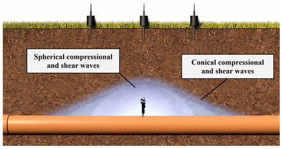
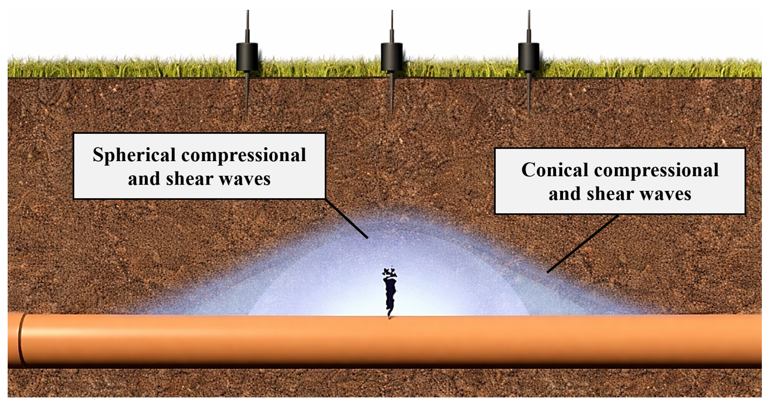
The vibro-acoustic signal generated by the leak propagates simultaneously through the pipe wall, the internal fluid, and the geomaterial, as ilustrated by Figure 1. At low frequencies, wave propagation in the pipe occurs predominantly through axisymmetric modes [34]. The radiation of this energy into the surrounding soil depends on the acoustic impedance ratio between the media. Since the wave propagation velocity in the pipe is higher than that in the geomaterial, the energy tends to be predominantly transmitted into the soil [35].
Figure 1.
Schematic diagram of wave propagation in the system.
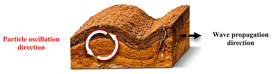
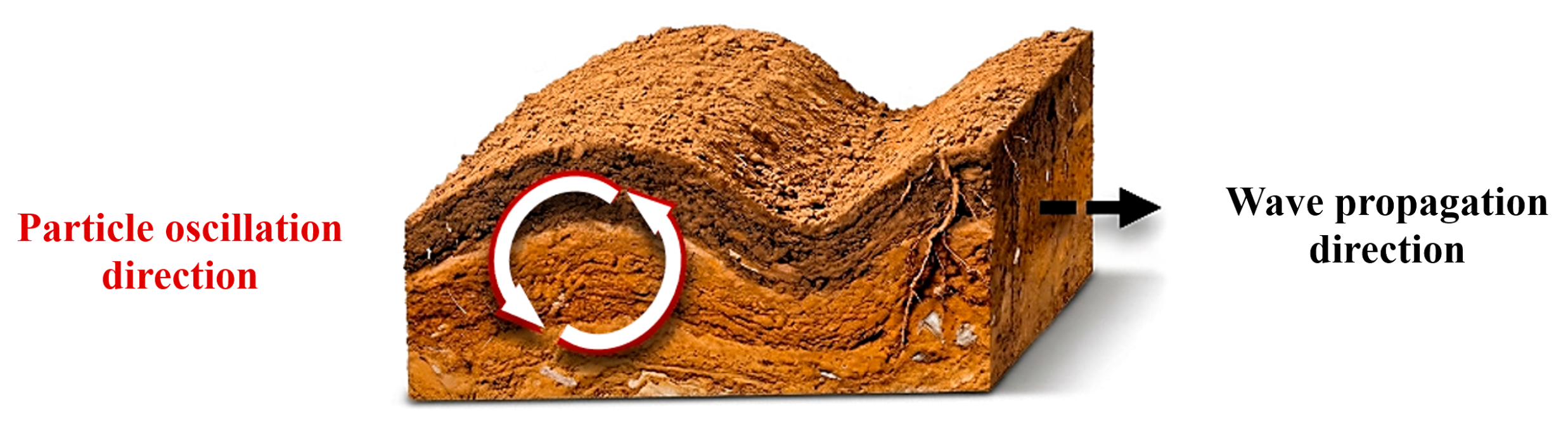
In the soil, the excitation propagates towards the surface through seismic body waves—namely compressional waves (P-waves) and shear waves (SV and SH), resulting from direct soil excitation—as well as conical refracted waves (compressional and shear) radiating from the pipe–soil interface [36]. As these waves reach the free surface of the medium, body waves combine to form surface waves, such as Rayleigh and Love waves. As illustrated in Figure 2, Rayleigh waves, resulting from the coupling between P and SV waves, exhibit retrograde elliptical motion and induce successive vertical surface displacements [37].
Figure 2.
Characteristics of Rayleigh surface waves.
The detectability of these signals at the surface is limited by seismic damping, mainly due to geometric spreading and attenuation—both intrinsic and apparent [38]. Therefore, accurate estimation of the leak location depends not only on the intensity of the signal generated in the subsurface, but also on the propagation conditions and the constraints imposed by the system as a whole. Structural and operational parameters of the network, as well as leak characteristics, also influence the signal power and its spectral content [39].
An integrated understanding of these phenomena is therefore essential for the development of more robust solutions. In this context, as will be discussed in Section 3, the present work investigates the energy decay in frequency bands as a function of the distance from the source, as a feature to be explored by machine learning models for leak localization.
3. Materials and Methods
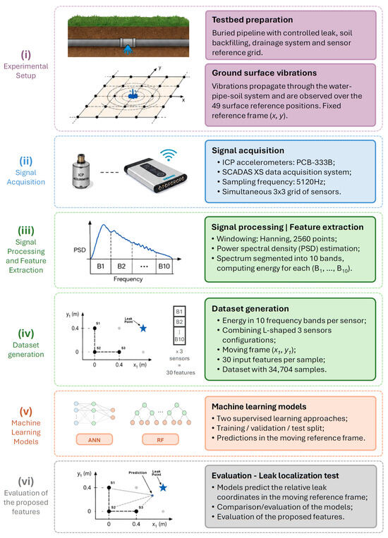
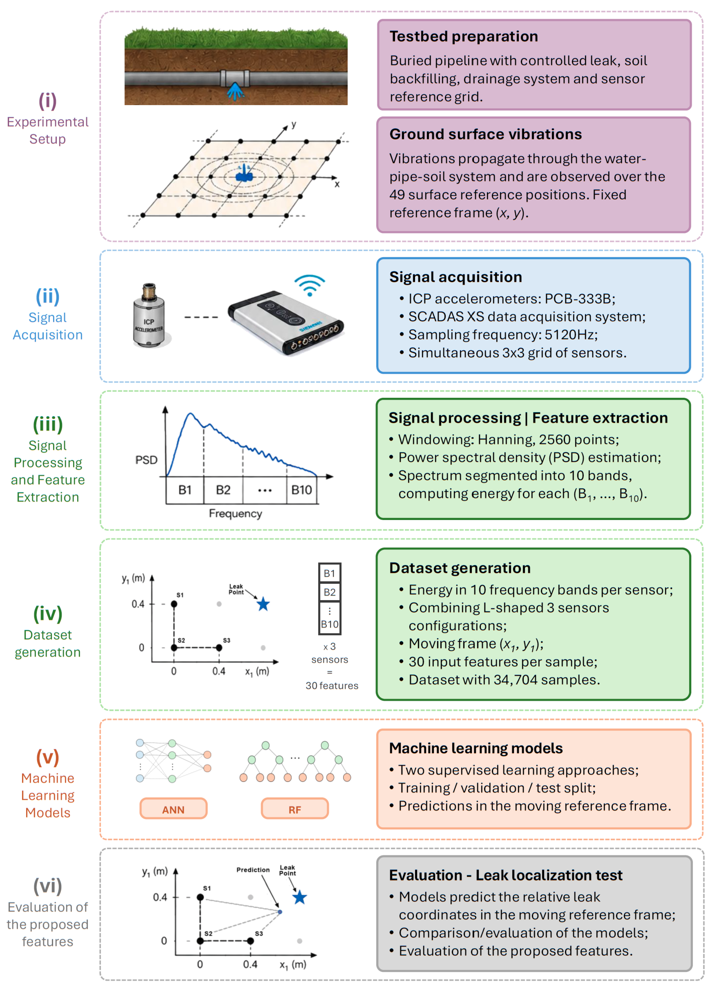
The methodology adopted in this study comprises six main stages: (i) development of an experimental testbed under controlled conditions; (ii) acquisition of leak-induced ground-surface vibration signals using a movable sensor array; (iii) signal processing and extraction of frequency-band energy features; (iv) generation of a dataset based on multiple L-shaped sensor configurations and moving-reference-frame coordinates; (v) training of two supervised machine-learning models; and (vi) evaluation of their capability to estimate leak location using the proposed feature set. Figure 3 summarizes the overall workflow adopted in this work.
Figure 3.
Overview of the workflow adopted to investigate the use of frequency-band energy features and machine-learning models for leak localization.
The methodology stages illustrated in Figure 3 are grouped and described in the following subsections. The discussion begins with the development of the experimental testbed used to generate the leak-induced vibration signals analyzed throughout this study.
3.1. Experimental Setup
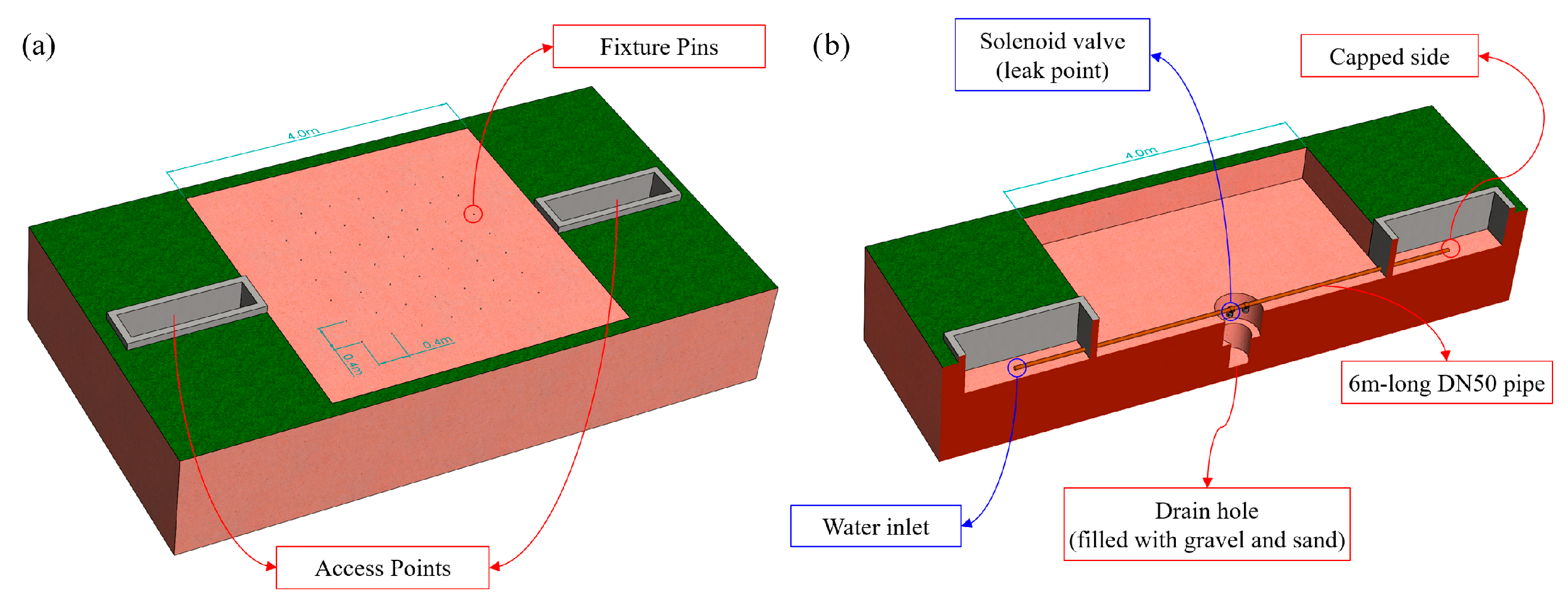
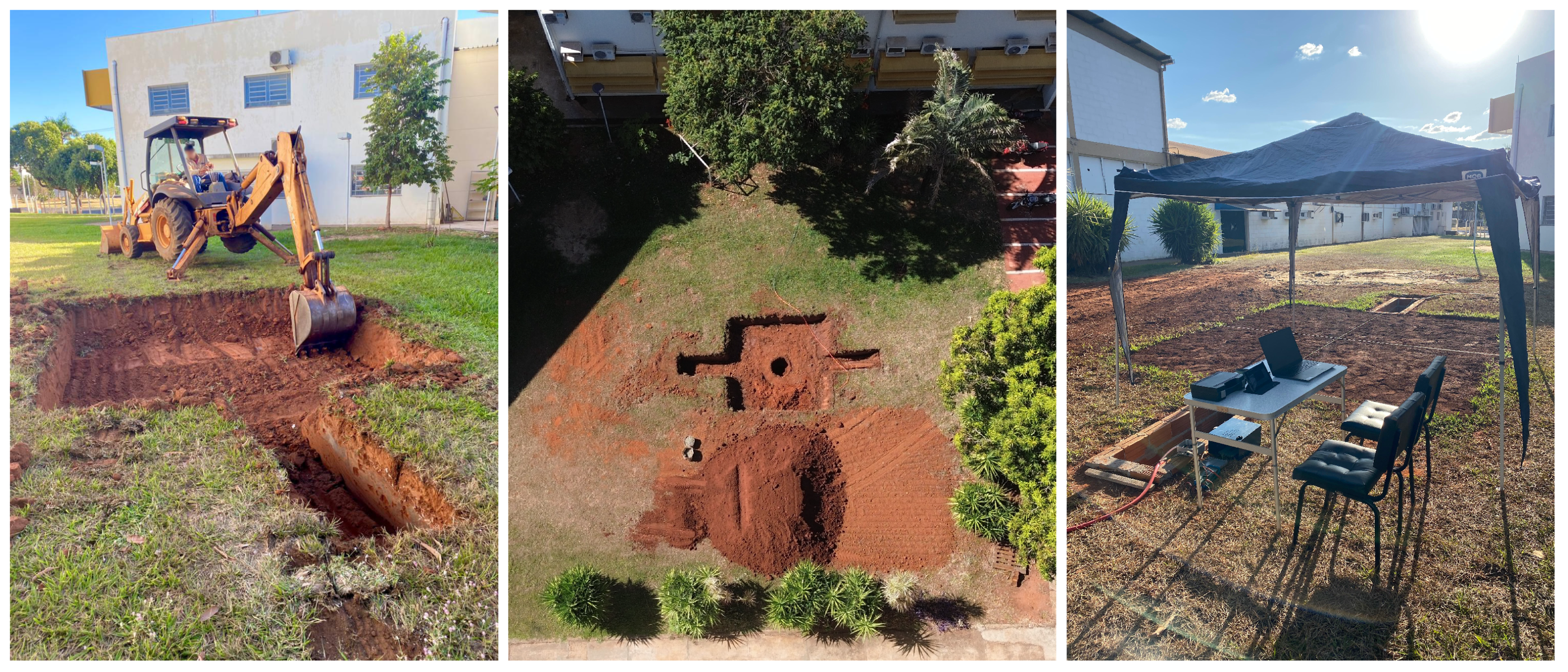
The experimental testbed used in this study was recently developed at the School of Engineering of São Paulo State University, in Ilha Solteira. It consists of a 6 m long polyvinyl chloride (PVC) pipe (50 mm diameter, 3 mm wall thickness) buried at a depth of 0.5 m. One capsule was installed at the central region (at 4 m) with a solenoid valve to generate controlled leaks through a 3 mm diameter hole. The pipe was installed in a trench approximately 8 m long and 0.8 m wide, and 0.5 m deep. A thin bedding layer was used for pipe support, following the recommendations of NBR 17015 [40], with gravel added locally to enhance drainage. Soil moisture sensors were installed around the pipe and drainage region to monitor saturation during experiments.
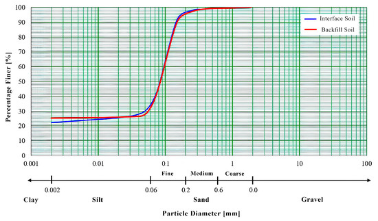
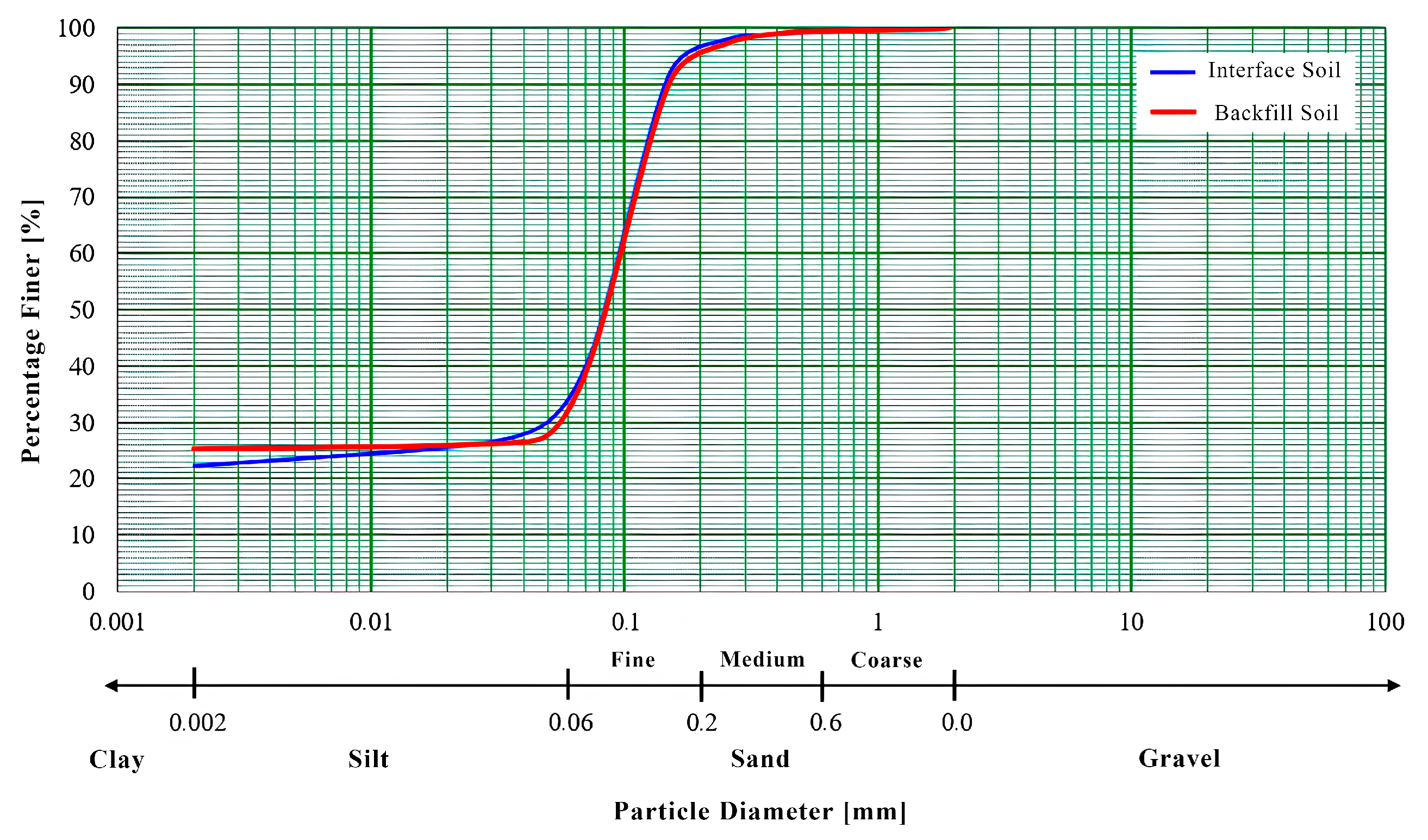
After installation, the trench was backfilled with soil similar to the original material and compacted in 0.1 m layers to ensure homogeneity. Figure 4 compares the particle size distributions of the native and backfill soils, while Table 1 summarizes their properties.
Figure 4.
Particle size distribution curves of the interface soil and the backfill soil.
Table 1.
Characterization of the soils at the testbed.
The soil consists of approximately 63% fine sand, 22∼25% of clay, and 7∼12% of silt, being classified as a slightly clayey fine sandy soil according to NBR 6502 [41]. Both soils exhibit similar properties, including the specific mass of approximately 2.74 g/cm3, and Atterberg limits (liquid limit of 23% and a plastic limit of 16%) ensuring similar impedances for the soils.
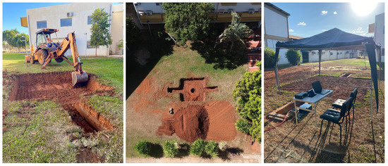
Unburied sections at both ends of the pipe were preserved to allow the connection of accessories such as manometers, valves, flow meters, and pressure regulators, enabling control of hydraulic conditions. Figure 5 and Figure 6 show the testbed during its design and construction stages.
Figure 5.
Testbed schematic: (a) complete view of the final configuration; (b) cross-sectional view showing buried components.
Figure 6.
Testbed views under its construction stage.
The experimental setup used during the data acquisition stage consisted of nine uniaxial piezoelectric ICP accelerometers (PCB 333B, nominal sensitivity of 100 mV/g) connected to a LMS SCADAS XS data acquisition system capable of simultaneously acquiring up to twelve channels. The SCADAS XS also provided the ICP signal conditioning required by the nine accelerometers. The acquisition system was operated in tablet mode using the TestLab Scope application, allowing wireless configuration and battery-powered operation during field measurements. Table 2 summarizes the main characteristics of the data acquisition setup.
Table 2.
Main characteristics of the data acquisition setup used during the experimental campaign.
For all acquisitions performed during the experimental campaign, a sampling frequency of 5120 Hz was adopted. This value allowed signal analysis up to 2560 Hz in the frequency domain according to the Nyquist criterion [42]. The sampling frequency was selected considering that leak noise signals are typically concentrated below 1000 Hz, although this range may vary depending on the pipe–soil system characteristics and the leak geometry. In the literature, sampling frequencies between 5 kHz and 12 kHz are commonly adopted for leak studies [26].
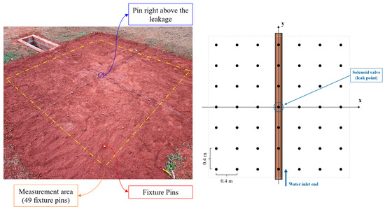
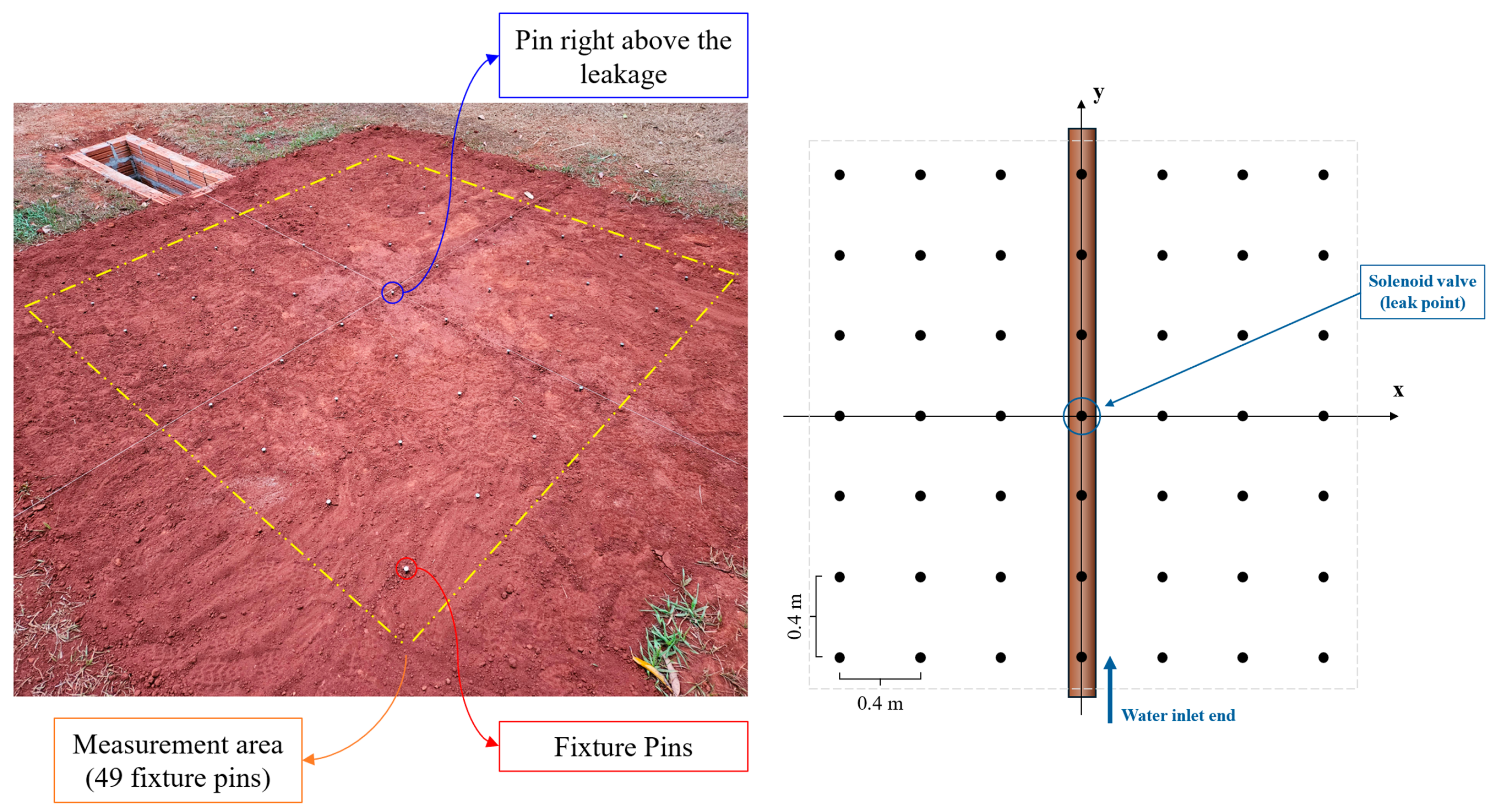
A grid composed of 7 × 7 measurement points was distributed over the ground surface, with uniform spacing of 0.40 m between adjacent points. The adopted spacing value was defined based on preliminary experimental considerations and on previous studies involving ground-surface vibration measurements above buried leaking pipes, such as the study by [19], which applied a 0.5 m spatial grid. In the present work, a slightly denser grid was selected to improve the representation of vibration attenuation patterns used as input features for the machine learning models.
Ferromagnetic pins were used to mount the sensors to the ground surface, taking advantage of the neodymium magnets integrated into the accelerometer connectors. This mounting approach was selected based on the recommendations of the PCB 333B Installation and Operating Manual, as it enables rapid sensor repositioning while maintaining adequate transmissibility and low mounting-induced attenuation for frequencies below 5 kHz [43].
The central point of the grid was positioned directly above the central section of the buried pipe with the remaining points distributed both parallel and perpendicular to the pipe axis. A coordinate system was defined to facilitate data organization, with the y-axis aligned with the pipe direction and the x-axis perpendicular to it. Figure 7 shows the sensor mounting and the measurement grid with the adopted coordinate system.
Figure 7.
Layout of the sensor fixing pins and defined reference system.
Once the sensor positions were defined, the water inlet was connected to the pipe end located at () to pressurize the system, as shown in Figure 7, while the opposite end remained sealed. The pipeline was pressurized using the municipal water supply, which is maintained by storage reservoirs with a head level above 27 mWC.
During all the experimental runs, the internal pressure was kept constant at approximately 248 kPa by a pressure regulating valve, ensuring consistent conditions across measurements. At this pressure, the leak flow rate remained stable at around 6.8 L/min.
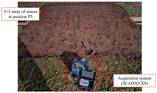
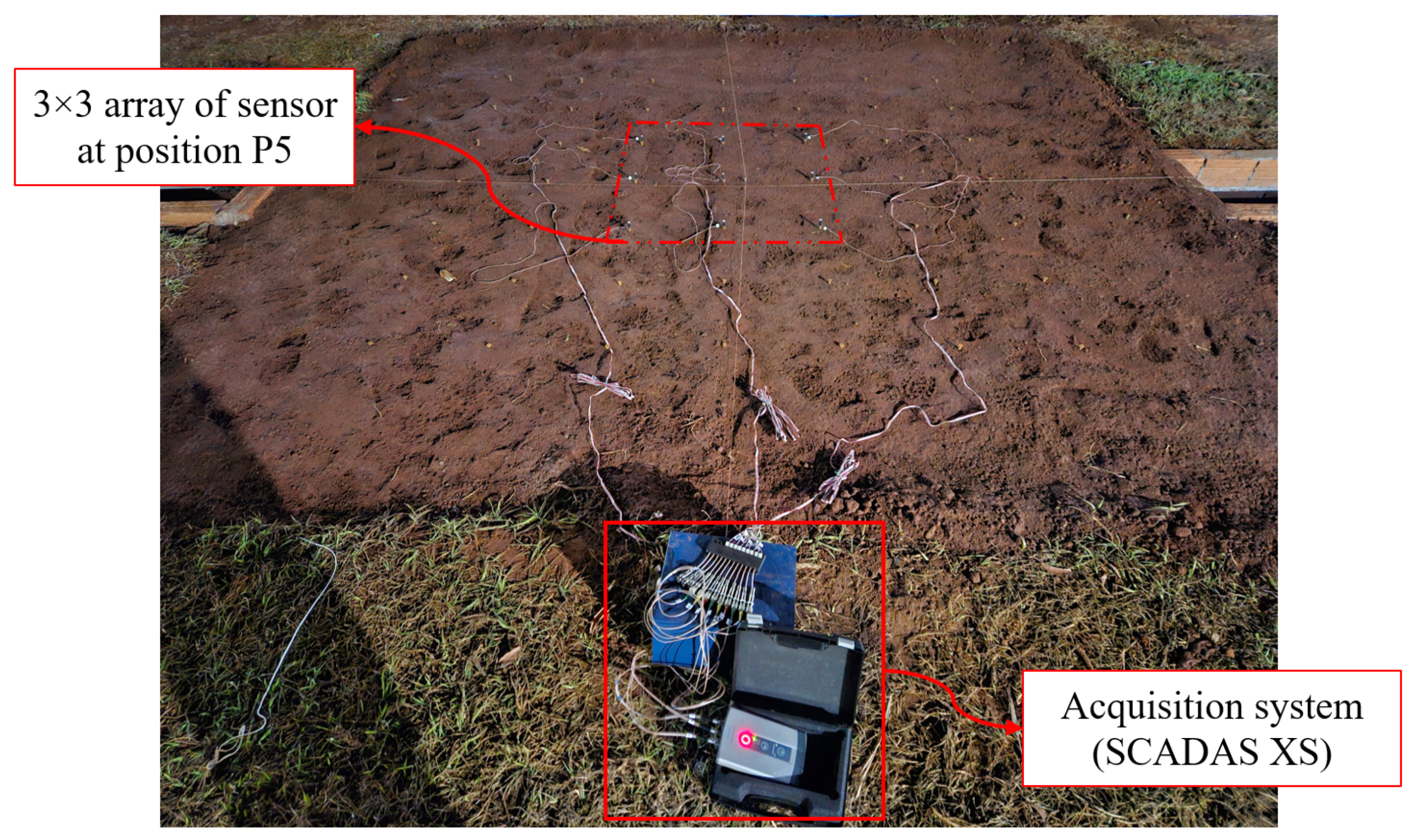
For each of the nine sensor array positions on the ground surface, one minute of data was collected while the leak was active. Additionally, an extra ten seconds of data were recorded under no-leak conditions at each position to provide a reference for background noise. Figure 8 shows the experimental setup during data acquisition at position P5, the central position where sensor A5 was located directly above the leak source.
Figure 8.
Experimental setup during one of the data acquisition measurements at the central position.
It is worth noting that, to minimize the influence of environmental noise and hydraulic disturbances associated with water consumption, all measurements were conducted during nighttime periods, following common operational practices adopted in acoustic leak detection activities.
3.2. Signal Processing and Feature Extraction
Since this study aims to evaluate the energy decay across frequency bands as a function of distance and direction from the source, the collected data at each measurement position were combined accordingly. To enable the comparison of energy decay along at least two directions, groups of three sensors were arranged in an “L-shaped” arrangement.
The adopted L-shaped sensor configuration was selected to introduce local bidirectional spatial information into the feature extraction process while maintaining a relatively simple acquisition setup. Using three neighboring sensors in a non-collinear arrangement allows the models to capture relative attenuation patterns along two orthogonal directions simultaneously, reducing potential ambiguities associated with one-dimensional spatial representations based on linear sensor pairs.
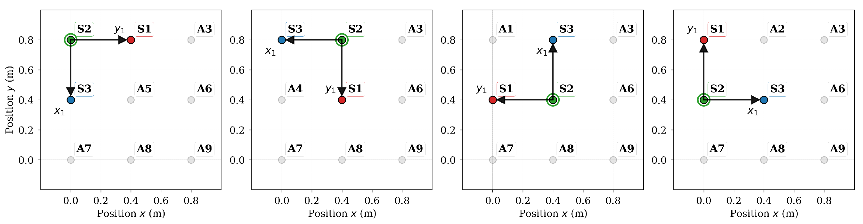
During the experiments, the physical leak location was kept fixed underground, while different L-shaped sensor configurations were arranged across the measurement grid. Consequently, each sensor configuration defines its own local coordinate system, and the same physical leak is represented by different relative coordinates depending on the position and orientation of the sensor trio. This moving-reference-frame approach was adopted to better represent practical leak-localization scenarios, where the position and orientation of the deployed sensors are known, whereas the leak position is unknown and must be estimated relative to the measurement system.
For each sensor trio, a moving reference frame () was defined, with sensor S2 at the origin, sensor S1 aligned along the axis, and sensor S3 along the axis. This configuration resulted in 16 possible L-shaped sensor combinations for each measurement position of the 3 × 3 grid. Figure 9 illustrates four representative examples of these combinations, highlighting the orientation of the moving reference frame according to the selected sensor trio.
Figure 9.
Examples of L-shaped sensor combinations and the corresponding moving reference frame orientation.
To relate the coordinates of sensor S2 from the inertial frame to the moving frame, the transformation matrix shown in Equation (1) was applied:
where x and y are the coordinates of sensor S2 in the inertial reference frame, and are the corresponding coordinates expressed in the moving frame, and is the counterclockwise rotation angle between the two coordinate systems.
This transformation allows all sensor configurations to be represented within a common local reference frame, regardless of their orientation within the measurement grid. The nine sensor array positions, combined with the 16 possible L-shaped configurations at each location, resulted in a total of 144 measurement configurations, ensuring a well-distributed dataset across the domain. In the local reference frame (), the relative position of the leak source with respect to the L-shaped sensor vertex spans from () to ().
After data acquisition, the acceleration signals were grouped into sensor trios, and the next step consisted of feature extraction for machine learning. Once the main objective was to quantify energy decay across frequency bands as a descriptor of source location, a straightforward approach would be to use the full amplitude spectrum as input, as done in previous studies [44]. However, this leads to a high-dimensional input space, particularly for fine frequency resolutions associated with large FFT windows.
To avoid this, a more compact representation was adopted by computing the signal energy within discrete frequency bands. This approach is consistent with the expected power-law decay of energy with frequency, as reported in previous studies [45], and allows capturing the key physical behavior—namely, the faster attenuation at higher frequencies—while significantly reducing the number of input features.
Given the sampling frequency of 5120 Hz, the usable frequency range (according to the Nyquist theorem) extends up to 2560 Hz. This range was divided into ten frequency bands of 256 Hz each. For notation purposes, the ten frequency bands were identified as B1–B10, where B1 corresponds to the 0–256 Hz interval, B2 to 256–512 Hz, and so forth, up to B10. The energy of the k-th energy band was then computed as shown in Equation (2):
where is the energy associated with the k-th frequency band, represents the FFT magnitude at the i-th frequency bin, and and define the lower and upper limits of the k-th frequency band. Higher values of indicate a greater concentration of vibration energy within that frequency interval.
Based on this, the signals from each sensor in the L-shaped trios were transformed into the frequency domain using a Hanning window of 2560 points with 50% overlap [42]. For each windowed segment, the energy in ten frequency bands was computed according to Equation (2). This procedure was applied to all measurement configurations, resulting in a dataset of 34,704 input samples. The dataset partitioning for training and testing is described in the following subsection.
3.3. Machine Learning Models
Recent studies have shown growing interest in applying machine-learning techniques to problems related to the prevention and reduction in treated water losses in buried pipelines. By analyzing data from vibro-acoustic sensors, ML algorithms can detect anomalies such as leaks with high precision [46,47,48,49]. Different learning strategies have been explored for this purpose, ranging from conventional neural networks and ensemble methods to more complex deep-learning architectures. In recent studies, convolutional neural networks have demonstrated promising results for leak localization using vibration data, owing to their ability to automatically extract spatial patterns from large datasets [44]. However, such architectures typically involve a larger number of trainable parameters and generally higher computational complexity.
Conventional feedforward neural networks, in contrast, can still effectively model nonlinear relationships while requiring simpler architectures and lower computational cost. Moreover, ensemble methods such as RFs constitute another attractive alternative, offering robustness to noisy data, reduced susceptibility to overfitting, and greater interpretability than simpler approaches such as individual decision trees.
Since the objective of the present study was not to perform an exhaustive comparison among machine-learning algorithms, two widely used and conceptually distinct regression approaches were selected for evaluation: Artificial Neural Network and Random Forest. Together, these methods provide complementary perspectives, combining nonlinear function approximation capabilities with the robustness and interpretability of ensemble learning techniques, being great choices to evaluate to investigate the suitability of the proposed feature set for leak localization purposes.
Among ML techniques, Artificial Neural Networks have become widely used across a broad range of applications due to their ability to approximate complex functions. ANNs are inspired by biological neurons and consist of interconnected layers that process information. To apply an ANN effectively, key variables—known as hyperparameters (HPs)—must be selected, as these define the architecture and behavior of the network. Unlike trainable parameters, HPs are set by the user to configure the network before training begins [50].
The most common training approach for ANNs is supervised learning, which uses the backpropagation algorithm. This method adjusts the weights between neurons by comparing predicted and expected outputs, minimizing the error iteratively. For a comprehensive understanding of ANN parameters and best practices, the foundational work by [50] provides an excellent reference for both beginners and experts in the field.
To evaluate the performance of a neural network during and after training, several key metrics are typically considered. In regression problems, two commonly used loss functions are the Mean Absolute Error (MAE) and Mean Squared Error (MSE). The MAE provides a straightforward average of the absolute differences between predicted and actual values, as defined in Equation (3), while the MSE emphasizes larger errors by squaring the differences, as shown in Equation (4).
where represents the true value for the given dataset, is the corresponding value predicted by the model, and n is the number of input samples used for the performance evaluation.
A simple Artificial Neural Network was selected in order to evaluate the possibility of using signal decay at higher frequencies as a relevant feature for the input data of a network. The final network configuration consists of an input layer with 30 neurons, corresponding to the energy distribution across ten frequency bands for each of the three sensors. Two intermediate fully connected layers were defined, the first consisting of 128 neurons and the second of 64 neurons. The output layer has two neurons tasked with predicting the coordinates related to the position of sensor S2. The activation function used in all layers was ReLU, except for the output layer, where a linear activation function was applied, aligning with the regression nature of the task. A dropout rate of 0.1 was applied between the first and second fully connected layers, randomly setting to zero 10% of the connections between layers, improving generalization. The Adam optimizer was chosen, with MSE as the loss function, and a learning rate set to 0.001.
The dataset, created following the pre-processing steps described in the previous section, was normalized between 0 and 1. Both input and output data were normalized; however, for the input data, normalization was performed separately for each sensor trio. This normalization process is a common practice in machine learning, facilitating faster model convergence [50].
For training, the dataset was split randomly, allocating 20% for testing and the remaining 80% for training, of which 20% was reserved for validation. A maximum of 200 training epochs was set, with a batch size of 32. Additionally, an early stopping function was implemented, monitoring the MAE of the validation data and halting training if no improvement was observed after 20 consecutive epochs, thus saving the best weights for the model. Table 3 outlines the final hyperparameters defined for the ANN model.
Table 3.
Selected hyperparameters for the ANN model.
The second ML approach tested in this work was the Random Forest regressor, which has gained prominence for its robustness, ability to handle high-dimensional data, and resilience to overfitting. Random Forests are ensemble methods that construct multiple decision trees during training and aggregate their outputs to generate final predictions. This ensemble approach reduces model variance and improves generalization, making it suitable for tasks involving regression from noisy, real-world data [51].
Similar to the ANN, the RF algorithm was applied to predict the relative position of the leak (in both and directions) based on energy features extracted from vibration signals, as described in the previous section. The dataset used was the same as for the ANN, consisted of 34,704 input samples, with 30 features each, and randomly splitting into 80% for training and 20% for testing. However, in contrast to the ANN implementation, no normalization was applied, as Random Forests are scale-invariant to the input features. The RF model was configured with bootstrap aggregation, utilizing the full feature set at each split, and reached an average tree depth of approximately 21.
After training, it was used to predict the leak coordinates () on the test set, and its regression performance was evaluated using three standard metrics: MSE, Root Mean Squared Error (RMSE), and the coefficient of determination (R2). Furthermore, a feature importance analysis was conducted to identify the most influential inputs, revealing that specific frequency bands contributed more significantly to the model’s predictions.
In addition to the quantitative metrics, the predictive performance of both the ANN and the RF models was visually assessed to provide a spatial interpretation of their accuracy. This involved comparing the real versus predicted coordinates along each axis, as well as generating two-dimensional scatter plots that overlay the estimated and actual leak positions across the measurement grid in the moving frame. These visualizations offer an intuitive assessment of regression patterns and allow direct comparison of how each ML technique generalizes across the operational domain.
All procedures for data loading, feature extraction, model training, and evaluation were performed using Python (3.10.20) [52]. The Artificial Neural Network model was implemented using TensorFlow (2.21.0) with Keras API (3.12.1) [53], while the Random Forest model was developed using Scikit-learn (1.7.2) [54]. Additional data processing and visualization tasks were performed using Pandas (2.3.3) [55], NumPy (2.2.5) [56], and Matplotlib (3.10.8) [57]. The computations were executed on a Samsung 960XFH laptop (Samsung Electronics Co., Ltd., Suwon, Republic of Korea) running Windows 11, equipped with an Intel Core i9-13900H processor, operating at a base frequency of 2.6 GHz and 32 GB of 6000 MT/s DDR5 RAM.
4. Results and Discussion
4.1. Surface Vibration Characteristics
Before evaluating the performance of the machine learning models, an initial analysis of the measured signals was conducted to characterize the behavior of leak-induced ground surface vibrations. Understanding the spatial distribution of signal energy and its spectral content is essential to justify the use of frequency-band energy as input features for the predictive models.
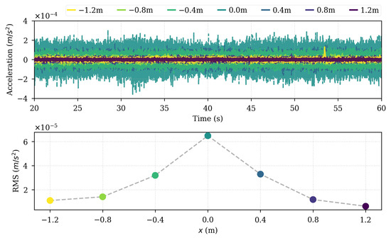
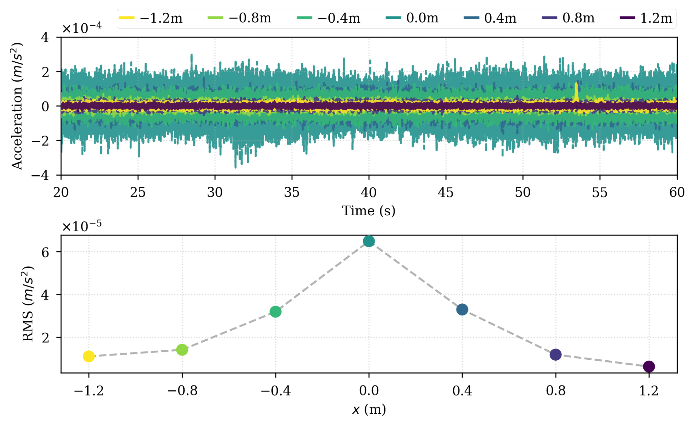
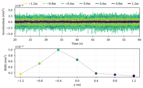
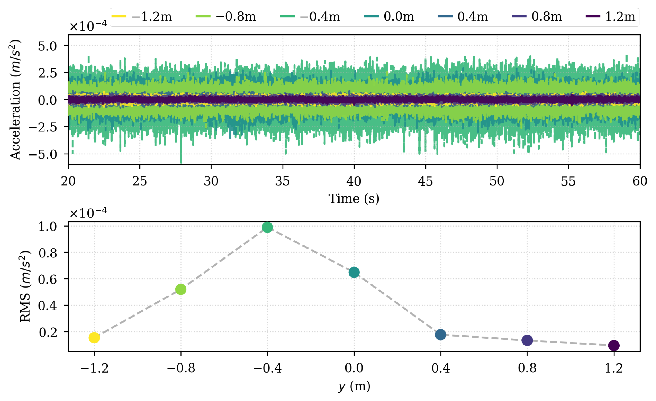
The first stage of the analysis focused on the decay of signal intensity with distance from the leak source. For this purpose, the root mean square (RMS) value of the acceleration signals was computed for all measurement positions. Figure 10 and Figure 11 present the RMS decay behavior for sensors positioned along the x-axis (perpendicular to the pipe) and the y-axis (parallel to the pipe), respectively.
Figure 10.
Energy decay of the signal for sensors positioned on the x-axis.
Figure 11.
Energy decay of the signal for sensors positioned on the y-axis.
For the sensors located along the x-axis, the time-domain signals exhibit relatively stable amplitudes during the acquisition period, with peak amplitudes on the order of m/s2. As expected, the RMS values decrease as the sensors move away from the leak position. A notable symmetry is observed between the RMS values measured at equivalent distances on the left and right sides of the pipeline, indicating that the attenuation pattern across the perpendicular direction is largely symmetric.
In contrast, the decay along the y-axis shows noticeable asymmetry. Although the RMS generally decreases with distance, the attenuation is less pronounced in the negative direction. In addition, the highest amplitude is not observed exactly at the origin but at a position located approximately m from the center. This behavior is attributed to the hydraulic conditions during the experiments. The water inlet was located at the pipe end corresponding to the negative y-direction, while the opposite end of the pipe remained closed. As a result, only the upstream region of the pipe experienced significant internal flow, while the downstream section remained nearly static despite being fully pressurized. This difference in flow conditions likely influenced the vibration energy transmitted to the surrounding soil, leading to stronger signals detected by sensors located upstream of the leak.
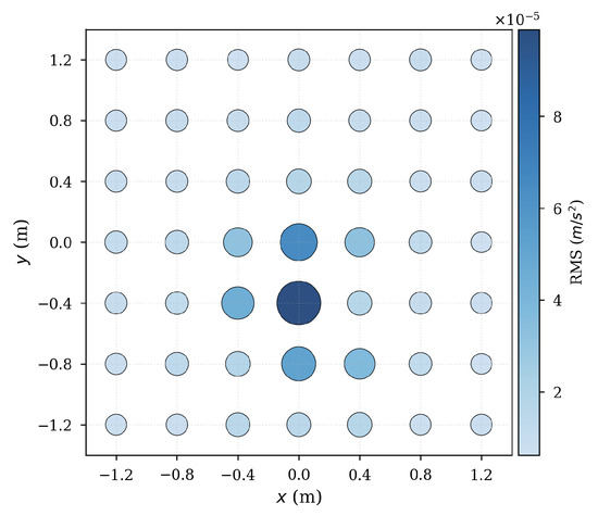
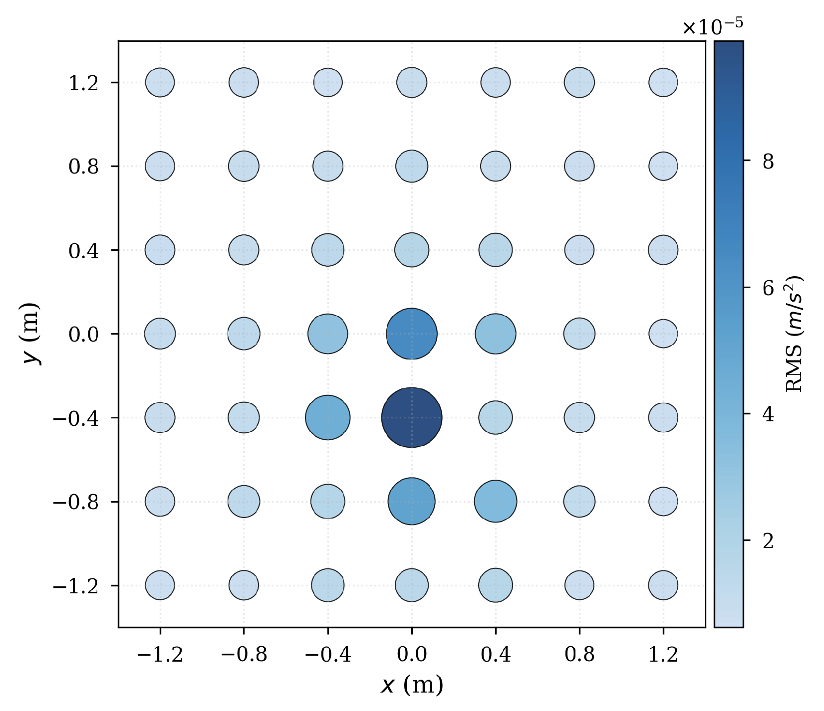
As shown in Figure 12, the global RMS map for all measurement points further confirms the overall attenuation trend. Signal intensity decreases progressively with increasing distance from the leak, stabilizing at distances greater than approximately m. Additionally, sensors located near the pipeline axis consistently register higher vibration levels than those located farther away.
Figure 12.
Spatial signal strength (RMS) for all measured positions.
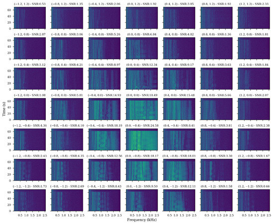
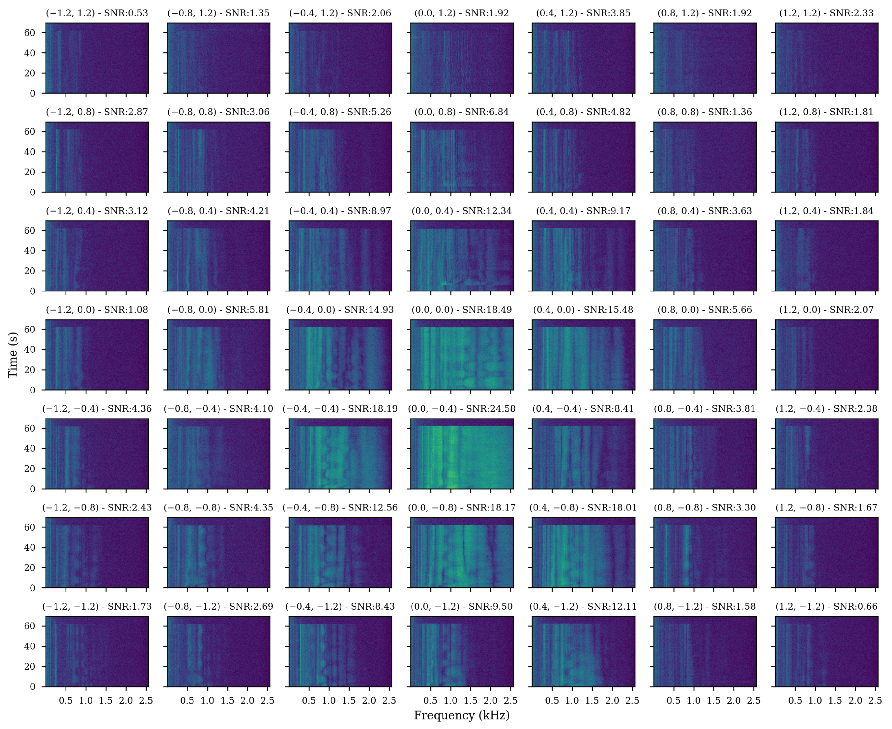
Although RMS analysis provides an overall indication of signal strength, it does not reveal how energy is distributed across the frequency spectrum. Previous studies have shown that soil acts as a low-pass filter for vibration propagation, attenuating higher frequencies more strongly than lower frequencies [36]. To investigate this effect, spectrograms were generated for all positions in the measurement grid, as shown in Figure 13.
Figure 13.
Spectrogram of the signals for each measurement positions within the 7 × 7 grid. All spectrograms share the same color scale, with brighter colors indicating higher spectral magnitude.
The spectrograms reveal a clear spectral attenuation pattern consistent with the expected low-pass filtering behavior of the soil. Lower frequencies retain a significant portion of the signal energy even at larger distances from the leak source, while higher frequency components rapidly decay as the propagation distance increases. This effect becomes particularly evident when comparing positions near the leak origin with those located at the edges of the measurement grid.
Signal-to-noise ratio (SNR) values were also estimated using the last ten seconds of each recording, during which the solenoid valve was closed and the leak was temporarily stopped. Because the background noise level remained nearly constant across the grid, the observed reduction in SNR at distant points can be attributed primarily to the attenuation of the leak-induced vibrations. This confirms that the signals recorded during the first 60 s of each measurement are effectively dominated by the leak source.
Another relevant observation from the spectrogram analysis is that the spectral characteristics of the leak signal resemble broadband noise, approaching the behavior of white noise, as previously reported in the literature [6]. Additionally, an oscillatory pattern in signal intensity can be observed within the frequency range between approximately 0.5 kHz and 1.5 kHz. Although the exact mechanism is not fully understood, this phenomenon may be associated with flow recirculation in the fluidized region near the leak jet [16].
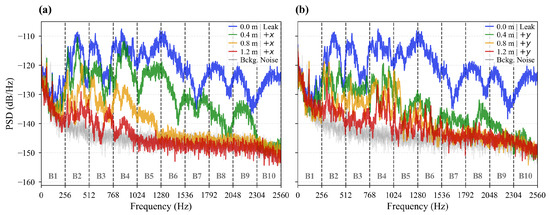
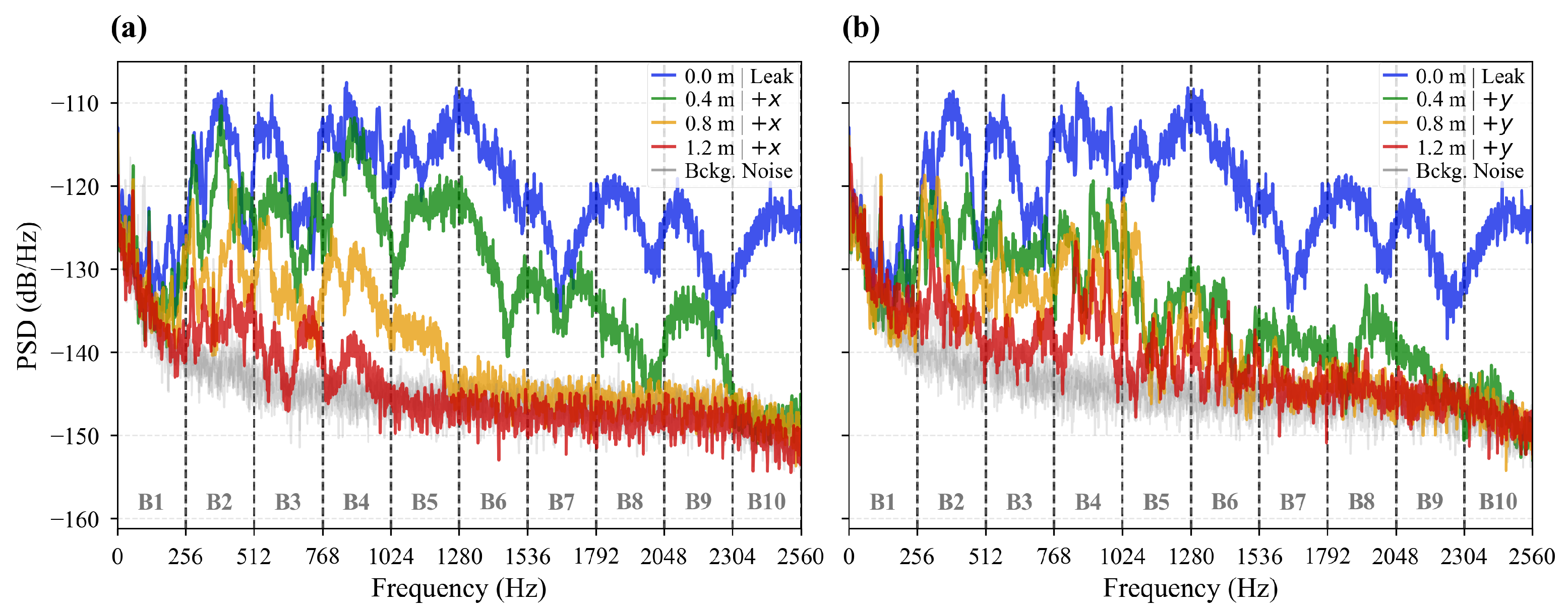
While the spectrogram matrix provides a comprehensive visualization of the spatial evolution of the spectral content over the entire measurement grid, the attenuation behavior can be observed more directly through power spectral density (PSD) comparisons at increasing distances from the leak source. Figure 14 presents representative PSDs for measured positions along both the x- and y-directions together with the background-noise spectrum obtained after leak interruption. The frequency-band limits adopted during the feature-extraction stage are also highlighted to facilitate the connection between the observed attenuation behavior and the descriptors used as inputs to the machine-learning models.
Figure 14.
Power spectral density (PSD) evolution with distance from the leak source along the (a) x- and (b) y-directions. Dashed vertical lines indicate the frequency-band boundaries adopted for feature extraction, while the background-noise spectrum is included for comparison. For both propagation directions, the spectrum measured at the position directly above the leak source is shown as the reference condition.
The PSD curves provide a more explicit visualization of the frequency-dependent attenuation phenomenon previously inferred from the spectrogram analysis. As the distance from the leak source increases, the higher-frequency components progressively decrease and, for the most distant measurement positions, approach the background-noise level, whereas lower-frequency components remain detectable over larger propagation distances. This behavior is observed in both propagation directions and is consistent with the low-pass filtering effect imposed by the soil.
Another important observation is that the attenuation is not uniform across the spectrum. Intermediate frequency ranges, particularly those corresponding to bands B2–B4, remain distinguishable over a substantial portion of the measurement grid while still exhibiting noticeable spatial variation with distance. In contrast, the lowest-frequency components tend to propagate over longer distances; however, the elevated background-noise levels observed within band B1 reduce the contrast between leak-induced vibrations and noise, limiting their usefulness as spatial descriptors for the proposed approach. Conversely, the highest-frequency components attenuate rapidly and become difficult to distinguish from background noise at larger distances. These results indicate that intermediate frequency bands provide a favorable balance between propagation capability and spatial sensitivity, preserving useful information about the relative position of the leak while remaining sufficiently robust to attenuation effects.
Overall, the RMS, spectrogram, and PSD analyses consistently demonstrate that the spatial decay of vibration energy varies significantly across frequency bands. This frequency-dependent attenuation behavior provides direct experimental support for representing the measured signals through their energy distribution across discrete frequency bands. Consequently, the adopted feature set offers a compact yet informative representation of the leak-induced vibrations under the investigated conditions, capturing both attenuation characteristics and spatial information relevant to the proposed leak-localization refinement task.
4.2. Comparative Performance of the Models
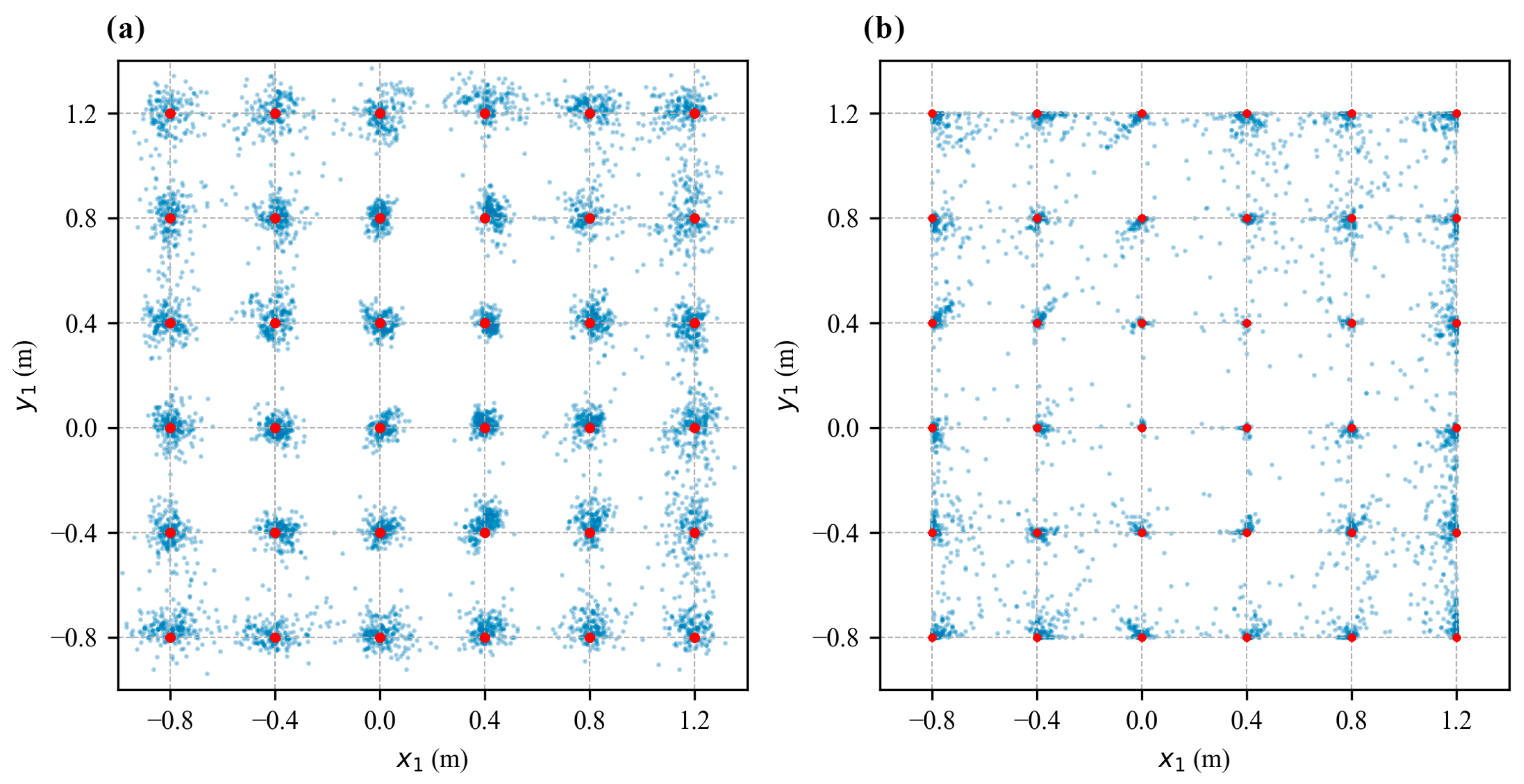
The predictive performance of the Artificial Neural Network and Random Forest models was evaluated using the test dataset. Figure 15 presents a two-dimensional spatial comparison between the actual and predicted leak positions for both models.
Figure 15.
Comparison between predicted and actual leak coordinates in the moving reference frame associated with each L-shaped sensor configuration: (a) ANN predictions; (b) RF predictions. Red markers indicate the actual relative leak coordinates (, ), whereas blue markers represent the corresponding model predictions.
It is important to note that the coordinates presented in Figure 15 are expressed in the moving reference frame previously defined in Section 3.2. Since the physical leak location remained fixed throughout the experiments, different leak coordinates were obtained by rotating and translating the sensor array across the measurement grid and expressing the leak position relative to the local coordinate system associated with each L-shaped sensor configuration. Consequently, the machine-learning models do not predict the absolute position of the leak within the experimental site, but rather its relative coordinates (, ) with respect to the sensor arrangement. This approach is consistent with practical field applications, where the position and orientation of the deployed sensors are known, whereas the leak location is unknown and must be estimated relative to the measurement system.
As can be observed, both models demonstrate strong agreement between predicted and actual leak positions, particularly for points located near the center of the measurement grid. In these regions, predictions are tightly clustered around the ground-truth coordinates, indicating that the models successfully capture the spatial patterns of the signals.
As the distance from the leak source increases, predictions become increasingly dispersed for both approaches. This behavior is consistent with the reduction in signal-to-noise ratio at larger distances, as previously discussed, which reduces the distinguishability of the vibration patterns associated with the leak. Additionally, the asymmetric distribution of signal intensity caused by the hydraulic conditions inside the pipe may introduces to localized deviations, particularly along the pipe axis.
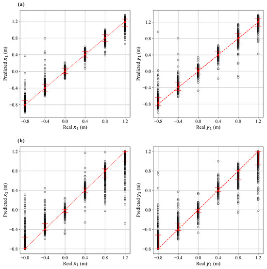
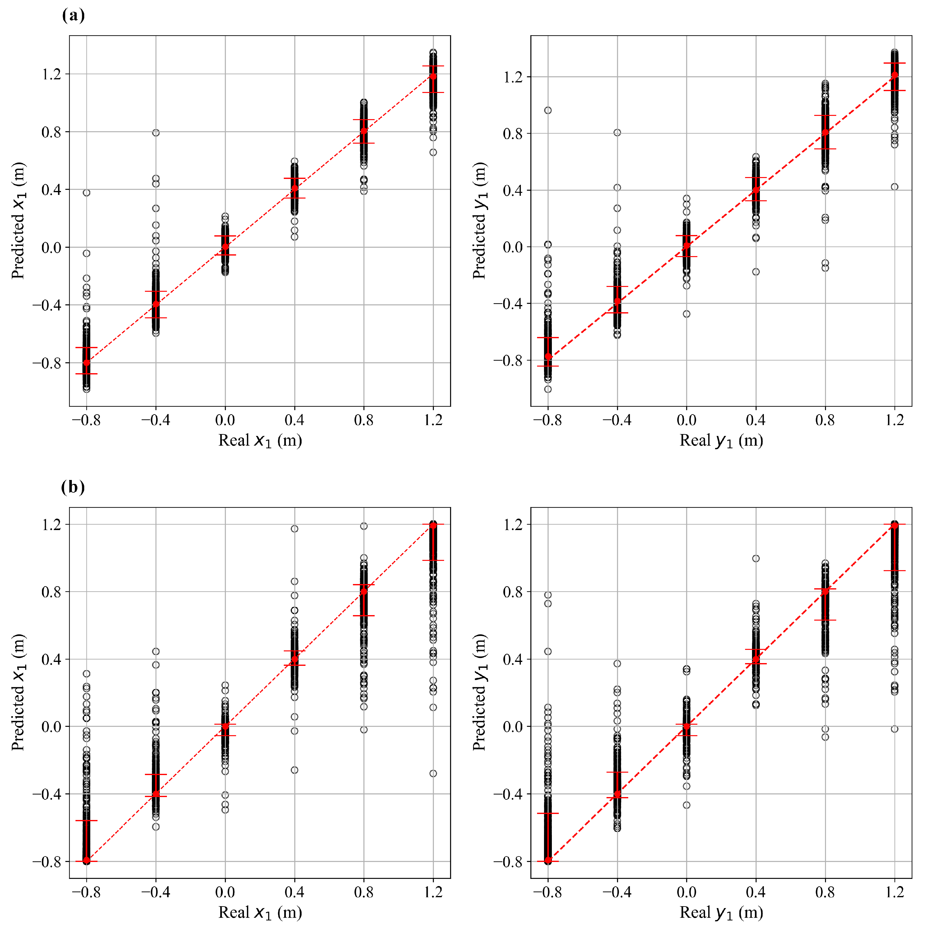
To further investigate the predictive behavior of the models presented in Figure 15, an axis-wise analysis was performed. Figure 16 presents the relationship between predicted and actual values for both spatial coordinates for the ANN and RF models.
Figure 16.
Axis-wise prediction analysis: (a) ANN predictions; (b) RF predictions. Black markers represent individual predictions, red markers indicate median predicted values, and error bars correspond to the 5th and 95th percentiles. The dashed red line represents the ideal identity relationship.
For both models, predictions are generally well aligned with the identity line, indicating that the relationship between input features and spatial position is consistently captured. In both cases, prediction dispersion increases toward the edges of the measurement grid, reflecting the reduced signal-to-noise ratio and lower vibration amplitudes at larger distances from the leak source.
Despite this increase in variability, the median predictions remain close to the ground-truth values across most of the domain, demonstrating stable central tendency. The ANN exhibits a slightly smoother distribution of predictions, consistent with its ability to approximate continuous nonlinear relationships. In contrast, the RF predictions show a more segmented behavior, consistent with the structure of decision-tree-based models.
An additional characteristic of the RF model is that all predictions remain bounded within the spatial limits of the training dataset. This behavior arises from its interpolation-based structure, which prevents extrapolation beyond the observed domain.
A quantitative comparison of the models is presented in Table 4. Both approaches achieved high coefficients of determination, exceeding 0.97 for all evaluated metrics, confirming the strong predictive capability of the proposed feature set.
Table 4.
Performance metrics of the ANN and RF models.
The RF model achieved lower mean absolute errors, both for individual axes and in terms of Euclidean distance, indicating superior average localization accuracy. In contrast, the ANN exhibited lower root mean squared errors and slightly higher coefficients of determination, suggesting greater robustness to larger prediction deviations. This difference reflects the distinct learning mechanisms of the models: while the RF relies on interpolation within the training domain, the ANN is capable of capturing smoother nonlinear relationships, which may reduce the impact of outliers.
From a practical perspective, the models exhibit complementary strengths. The RF model is better suited for scenarios where the search domain is well constrained and closely aligned with the training data, providing more accurate average estimates. In contrast, the ANN demonstrates greater stability in the presence of higher uncertainty, which may be advantageous under conditions with lower signal quality or deviations from the training distribution.
4.3. Feature Importance Analysis
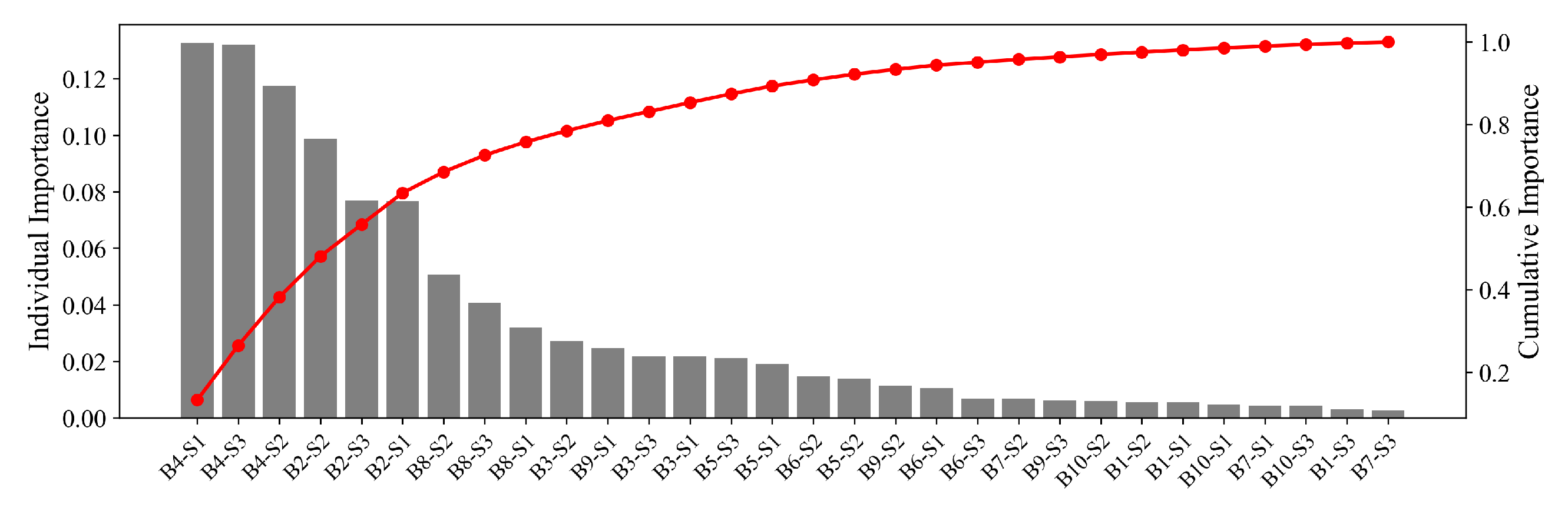
The Random Forest model also allows the quantification of the relative importance of the input features. Figure 17 presents the contribution of each frequency-band energy component to the model predictions.
Figure 17.
Feature importance ranking for the 30 input features used by the Random Forest model, corresponding to the energy values extracted from 10 frequency bands (B1–B10) for each sensor in the L-shaped sensor trio (S1, S2, and S3). Gray bars indicate the individual feature importance, while the red line with markers represents the cumulative importance.
The results indicate that mid-frequency bands contribute most significantly to the model predictions, with bands such as B4 (768 Hz–1024 Hz) and B2 (256 Hz–512 Hz) presenting the highest importance values. This observation is consistent with the physical behavior of vibro-acoustic wave propagation in soil. Mid-frequency components provide a balance between attenuation and spatial resolution: lower frequencies tend to propagate over longer distances but carry less spatial detail, while higher frequencies are more strongly attenuated and therefore contribute primarily in regions close to the leak source.
Although individual propagation modes were not isolated experimentally, the observed feature-importance distribution is consistent with the wave propagation mechanisms discussed in Section 2 and reported in the literature. Leak-induced vibrations reaching the ground surface are generally considered to be strongly influenced by Rayleigh-wave propagation [45], which tends to preserve lower-frequency components over longer distances, while higher-frequency components experience stronger attenuation within the pipe–soil system. Consequently, intermediate frequency bands appear to provide a favorable compromise between propagation capability and spatial sensitivity, which may explain their greater contribution to the RF predictions.
Overall, the analyses presented in this subsection reinforce the interpretations discussed along Section 4, providing additional insight into the learning behavior and predictive characteristics of the evaluated models applying the proposed input features.
4.4. Practical Considerations and Future Work
Although the experiments were conducted outdoors using a buried pipeline and natural soil, the testbed still represents a controlled environment. Real distribution networks may exhibit substantially greater complexity due to heterogeneous soil stratigraphy, pavement layers, buried utilities, vegetation roots, and other underground structures that can alter wave propagation paths and attenuation behavior.
Since the proposed feature-extraction approach relies on frequency-dependent attenuation patterns, its effectiveness is inherently influenced by the physical conditions governing vibration propagation. Variations in soil properties such as moisture content, density, porosity, and compaction may alter the spectral distribution of the measured vibrations, while differences in pipe material, burial depth, diameter, and operating pressure can further modify the observed signal characteristics. As a consequence, the ANN and RF models may experience performance degradation when applied to conditions that differ substantially from those represented in the training dataset. Future studies should therefore investigate multi-condition datasets covering a broader range of soil types, pipe characteristics, and operational scenarios, as well as strategies such as recalibration, transfer learning, and the incorporation of environmental descriptors (e.g., soil characteristics, pipe depth, and operating conditions) as auxiliary model inputs to improve transferability and robustness.
Environmental vibration sources such as road traffic, construction activities, industrial machinery, or pedestrian movement may introduce additional broadband components that overlap with leak-induced vibrations. Although the measured SNR values demonstrated that leak-generated signals were clearly distinguishable under the experimental conditions, the robustness of the proposed approach under highly contaminated acoustic environments remains an important topic for future investigation. Future studies may explore the use of temporal and frequency-domain filtering strategies to enhance the separation between leak-induced vibrations and external noise sources, particularly considering the relatively stationary nature of leak signals when compared with many transient environmental disturbances.
Despite these limitations, the results demonstrate that frequency-band energy descriptors preserve meaningful spatial information associated with leak position, even when measured indirectly through ground-surface vibrations. The high predictive performance achieved by both ANN and RF models indicates that frequency-dependent attenuation patterns can be effectively exploited as localization features. These findings support the feasibility of using spectral energy distributions as compact descriptors for leak localization and provide an experimental basis for future investigations under more complex environmental conditions. Furthermore, the proposed descriptors may be integrated with additional sensing modalities, complementary signal features, or alternative localization techniques to further improve localization accuracy, robustness, and applicability across different operational scenarios.
5. Conclusions
This work investigated the use of acceleration measurements collected at the ground surface, combined with machine learning techniques to estimate the location of leaks in buried pipelines. An experimental testbed was developed to simulate controlled leakage conditions and acquire vibration signals over a spatial measurement grid. Energy features extracted from discrete frequency bands were used as inputs for two regression models: an Artificial Neural Network and a Random Forest.
The signal analysis demonstrated that vibration amplitude decreases with distance from the leak source and that the soil acts as a low-pass filter, attenuating higher frequencies more strongly. These characteristics supported the use of frequency-band energy as a compact representation of the signal for localization purposes, which is conceptually consistent with conventional acoustic leak localization approaches that rely on listening devices to identify variations in sound intensity along the ground surface.
Both models demonstrated strong predictive performance. The RF achieved lower mean absolute errors, with a Euclidean MAE of 5.32 cm, indicating higher average localization accuracy. In contrast, the ANN produced lower root mean squared errors and slightly higher coefficients of determination. These results indicate that the RF provides higher average accuracy, whereas the ANN shows greater robustness to larger prediction deviations. In both cases, the high values confirm that the proposed features effectively encode spatial information, enabling accurate estimation of leak positions from surface vibration measurements under the experimental conditions investigated in this study.
Overall, the results demonstrate the potential of frequency-dependent attenuation patterns as descriptors for leak localization. The proposed combination of ground-surface vibration measurements and machine learning models achieved accurate predictions under the conditions investigated and provides a foundation for future validation under more realistic field conditions.
Author Contributions
Conceptualization, V.d.A.S., M.S.P. and O.S.; methodology, V.d.A.S., M.S.P. and O.S.; software, V.d.A.S.; validation, O.S.; formal analysis, V.d.A.S.; investigation, V.d.A.S., M.S.P., O.S., C.B.S. and K.d.S.R.; resources, O.S. and A.T.P.; data curation, V.d.A.S.; writing—original draft preparation, V.d.A.S.; writing—review and editing, O.S., A.T.P., M.S.P. and V.d.A.S.; visualization, V.d.A.S. and O.S.; supervision, O.S. and A.T.P.; funding acquisition, V.d.A.S., O.S. and A.T.P. All authors have read and agreed to the published version of the manuscript.
Funding
This study was financed in part by the Coordenação de Aperfeiçoamento de Pessoal de Nível Superior - Brasil (CAPES) - Finance Code 001. The first author is funded by CAPES with the grant 88887.915145/2023-00. This work was supported, in part, by the São Paulo Research Foundation (FAPESP) under grant number 24/13559-0 and 25/00583-3. This work has also received support from the Fundação de Ensino, Pesquisa e Extensão de Ilha Solteira (FEPISA).
Institutional Review Board Statement
Not applicable.
Informed Consent Statement
Not applicable.
Data Availability Statement
The data presented in this study are available on request from the corresponding author due to privacy.
Conflicts of Interest
The authors declare no conflicts of interest.
Abbreviations
The following abbreviations are used in this manuscript:
| ANN | Artificial Neural Network |
| FFT | Fast Fourier Transform |
| GPR | Ground-Penetrating Radar |
| HP | Hyperparameter |
| ICP | Integrated Circuit Piezoelectric |
| LSTM | Long Short-Term Memory |
| MAE | Mean Absolute Error |
| ML | Machine Learning |
| MSE | Mean Squared Error |
| MTU | Mapping the Underworld |
| PVC | Polyvinyl Chloride |
| RF | Random Forest |
| RMS | Root Mean Square |
| RMSE | Root Mean Squared Error |
| SNR | Signal-to-Noise Ratio |
Appendix A. ANN Training Convergence
The training process of the ANN was evaluated by analyzing the convergence of the loss function. Figure A1 presents the evolution of the MSE and MAE during training.
Figure A1.
ANN convergence curves for training and validation datasets.
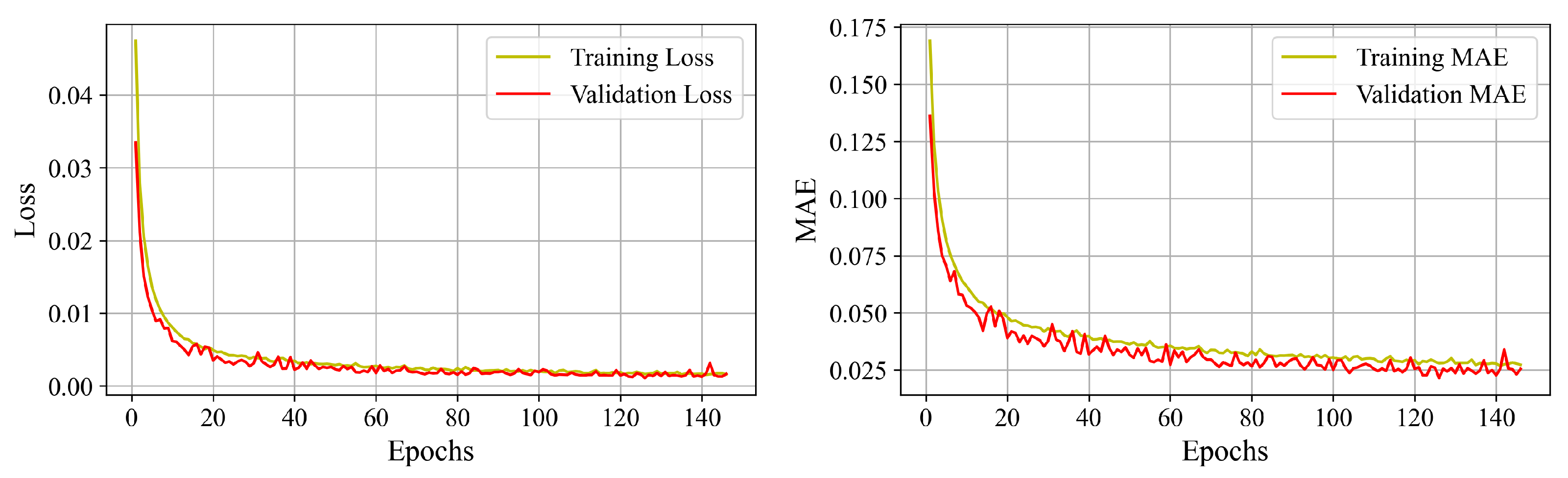
Both curves exhibit a rapid reduction during the initial training stage, particularly within the first epochs, indicating efficient learning of the underlying input–output relationships. After this phase, the curves progressively stabilize, suggesting convergence of the optimization process. The close agreement between training and validation curves throughout the training indicates that overfitting was effectively controlled. The early stopping mechanism halted the training at epoch 146, with the optimal model obtained at epoch 126, corresponding to the minimum validation loss.
References
- Hu, Z.; Tariq, S.; Zayed, T. A comprehensive review of acoustic based leak localization method in pressurized pipelines. Mech. Syst. Signal Process. 2021, 161, 107994. [Google Scholar] [CrossRef]
- Romero-Ben, L.; Alves, D.; Blesa, J.; Cembrano, G.; Puig, V.; Duviella, E. Leak detection and localization in water distribution networks: Review and perspective. Annu. Rev. Control 2023, 55, 392–419. [Google Scholar] [CrossRef]
- Bakhtawar, B.; Zayed, T. Review of Water Leak Detection and Localization Methods through Hydrophone Technology. J. Pipeline Syst. Eng. Pract. 2021, 12, 03121002. [Google Scholar] [CrossRef]
- Yu, Y.; Shi, P.; Krynkin, A.; Horoshenkov, K.V. An application of a beamforming technique, linear acoustic array and robot for pipe condition localization. Measurement 2024, 238, 115361. [Google Scholar] [CrossRef]
- Yu, Y.; Safari, A.; Niu, X.; Drinkwater, B.; Horoshenkov, K.V. Acoustic and ultrasonic techniques for defect detection and condition monitoring in water and sewerage pipes: A review. Appl. Acoust. 2021, 183, 108282–108295. [Google Scholar] [CrossRef]
- Scussel, O.; Brennan, M.J.; Almeida, F.C.L.; Muggleton, J.M.; Rustighi, E.; Joseph, P.F. Estimating the spectrum of leak noise in buried plastic water distribution pipes using acoustic or vibration measurements remote from the leak. Mech. Syst. Signal Process. 2021, 147, 107059. [Google Scholar] [CrossRef]
- Hamilton, S.; Charalambous, B. Leak Detection: Technology and Implementation; IWA Publishing: London, UK, 2013. [Google Scholar] [CrossRef][Green Version]
- El-Zahab, S.; Zayed, T. Leak detection in water distribution networks: An introductory overview. Smart Water 2019, 4, 5. [Google Scholar] [CrossRef]
- Dutta, R.; Cohn, A.G.; Muggleton, J.M. 3D mapping of buried underworld infrastructure using dynamic Bayesian network based multi-sensory image data fusion. J. Appl. Geophys. 2013, 92, 8–19. [Google Scholar] [CrossRef]
- Muggleton, J.M.; Rustighi, E. ‘Mapping the Underworld’: Recent developments in vibro-acoustic techniques to locate buried infrastructure. Géotechnique Lett. 2013, 3, 137–141. [Google Scholar] [CrossRef]
- Liu, Y.; Habibi, D.; Chai, D.; Wang, X.; Chen, H.; Gao, Y.; Li, S. A Comprehensive Review of Acoustic Methods for Locating Underground Pipelines. Appl. Sci. 2020, 10, 1031. [Google Scholar] [CrossRef]
- Jette, A.; Parker, J. Surface displacements accompanying the propagation of acoustic waves within an underground pipe. J. Sound Vib. 1980, 69, 265–274. [Google Scholar] [CrossRef]
- Krylov, V. Generation of Low-Frequency Ground Vibrations by Sound Waves Propagating in Underground Gas Pipes. J. Low Freq. Noise Vib. Act. Control 1995, 14, 143–149. [Google Scholar] [CrossRef]
- de Barros, F.C.P.; Luco, J.E. Seismic response of a cylindrical shell embedded in a layered viscoelastic half-space. II: Validation and numerical results. Earthq. Eng. Struct. Dyn. 1994, 23, 569–580. [Google Scholar] [CrossRef]
- Gao, Y.; Muggleton, J.M.; Liu, Y.; Rustighi, E. An analytical model of ground surface vibration due to axisymmetric wave motion in buried fluid-filled pipes. J. Sound Vib. 2017, 395, 142–159. [Google Scholar] [CrossRef]
- Zhang, P.; He, J.; Huang, W.; Yuan, Y.; Wu, C.; Zhang, J.; Yuan, Y.; Wang, P.; Yang, B.; Cheng, K.; et al. Ground vibration analysis of leak signals from buried liquid-filled pipes: An experimental investigation. Appl. Acoust. 2022, 200, 109054. [Google Scholar] [CrossRef]
- Muggleton, J.; Brennan, M. The design and instrumentation of an experimental rig to investigate acoustic methods for the detection and location of underground piping systems. Appl. Acoust. 2008, 69, 1101–1107. [Google Scholar] [CrossRef]
- Muggleton, J.; Brennan, M.; Gao, Y. Determining the location of buried plastic water pipes from measurements of ground surface vibration. J. Appl. Geophys. 2011, 75, 54–61. [Google Scholar] [CrossRef]
- Scussel, O.; Brennan, M.; Iwanaga, M.; Almeida, F.; Karimi, M.; Muggleton, J.; Joseph, P.; Rustighi, E. Analysis of phase data from ground vibration measurements above a leaking plastic water pipe. J. Sound Vib. 2023, 564, 117873. [Google Scholar] [CrossRef]
- Muggleton, J.; Papandreou, B. A shear wave ground surface vibration technique for the detection of buried pipes. J. Appl. Geophys. 2014, 106, 164–172. [Google Scholar] [CrossRef]
- Yan, S.; Yuan, H.; Gao, Y.; Jin, B.; Deng, L.; Li, K. Suppression of the influence of surface waves on shear wave imaging for buried pipe location. J. Appl. Geophys. 2022, 196, 104517. [Google Scholar] [CrossRef]
- Cui, X.; Gao, Y.; Muggleton, J.; Liu, Y. Superimposed imaging of acoustic wave reflections for the detection of underground nonmetallic pipelines. Mech. Syst. Signal Process. 2024, 209, 111127. [Google Scholar] [CrossRef]
- Qi, Y.; Wang, X.; Yang, X.; Sun, T.; Razzaq, I.; Yang, L.; Wang, Y.; Rasool, G. Nonexcavation Localization Method for Buried PE Pipes Based on Elastic Wave Reflection Imaging and the BPA Method. IEEE Sens. J. 2024, 24, 17987–17998. [Google Scholar] [CrossRef]
- Qi, Y.; Wang, X.; Yang, L.; Wang, Y.; Guo, Z. A non-excavation detection method for buried PE pipelines based on 3D time-domain stacking focusing of elastic wave reflection. Meas. Sci. Technol. 2023, 35, 025120. [Google Scholar] [CrossRef]
- Qi, Y.; Wang, X.; Yang, X.; Sun, T.; Razzaq, I.; Yang, L.; Wang, Y.; Rasool, G. Research on acoustic methods for buried PE pipeline detection based on LSTM neural networks. Meas. Sci. Technol. 2024, 35, 096001. [Google Scholar] [CrossRef]
- Scussel, O.; Brennan, M.J.; Muggleton, J.M.; de Almeida, F.C.L.; Joseph, P.F.; Gao, Y. An Investigation into the Physical Mechanisms of Leak Noise Propagation in Buried Plastic Water Pipes: A Wave Dynamic Stiffness Approach. Acoustics 2024, 6, 157–176. [Google Scholar] [CrossRef]
- Pollock, A.; Hsu, S.Y. Leak detection using acoustic emission. J. Acoust. Emiss. 1982, 1, 237–243. [Google Scholar]
- Thompson, M.; Chapman, C.; Howison, S.; Ockendon, J. Noise generation by water pipe leaks. In Proceedings of the 40th European Study Group with Industry, Keele, UK, 9–12 April 2001; pp. D1–D6. [Google Scholar]
- Papastefanou, A.S.; Joseph, P.F.; Brennan, M.J. Experimental Investigation into the Characteristics of in Pipe Leak Noise in Plastic Water Filled Pipes. Acta Acust. United Acust. 2012, 98, 847–856. [Google Scholar] [CrossRef]
- Ross, D. Mechanics of Underwater Noise; Pergamon Press Inc.: Los Angeles, CA, USA, 1976; p. 375. [Google Scholar]
- Miller, R.K.; Pollock, A.A.; Watts, D.J.; Carlyle, J.M.; Tafuri, A.N.; Yezzi, J.J., Jr. A reference standard for the development of acoustic emission pipeline leak detection techniques. NDT&E Int. 1999, 32, 1–8. [Google Scholar] [CrossRef]
- Novak, J.A. Cavitation and Bubble Formation in Water Distribution Systems. Master’s Thesis, Virginia Polytechnic Institute and State University, Blacksburg, VA, USA, 2005. [Google Scholar]
- Zohora, F. Study of Pipe Leak Fluid Dynamic Characteristics and Their Influences on Acoustic Emission Generation. Ph.D. Thesis, Queensland University of Technology, Brisbane, Australia, 2020. [Google Scholar]
- Brennan, M.J.; Chapman, D.N.; Joseph, P.F.; Metje, N.; Muggleton, J.M.; Rustighi, E. Achieving Zero Leakage by 2050: Leak Detection and Location Methods—Acoustic Leak Detection; Technical report; UK Water Industry Research Limited: London, UK, 2017. [Google Scholar]
- Muggleton, J.M.; Scussel, O.; Rustighi, E.; Brennan, M.J.; Almeida, F.; Karimi, M.; Joseph, P.F. A simplified Model of the Ground Surface Vibration Arising from a Leaking Pipe. In Proceedings of the Recent Trends in Wave Mechanics and Vibrations; Dimitrovová, Z., Biswas, P., Gonçalves, R., Silva, T., Eds.; Springer: Cham, Switzerland, 2023; Volume 125. [Google Scholar] [CrossRef]
- Proença, M.S.; Paschoalini, A.T.; Silva, J.B.C.; Souza, A.; Obata, D.H.S.; Lima, L.P.M.; Boaventura, O.D.Z. The Finite Element Method applied in the viscoelastic constitutive model of Kelvin–Voigt for characterization of the soil dynamic response to water leakage simulation. J. Braz. Soc. Mech. Sci. Eng. 2022, 44, 470. [Google Scholar] [CrossRef]
- Rayleigh, L. On waves propagated along the plane surface of an elastic solid. Proc. Lond. Math. Soc. 1885, 1, 4–11. [Google Scholar] [CrossRef]
- Liner, C.L. Elements of Seismic Dispersion: A Somewhat Practical Guide to Frequency-Dependent Phenomena; Number 15 in Distinguished Instructor Series; Society of Exploration Geophysicists (SEG): Houston, TX, USA, 2012; p. 184. [Google Scholar]
- Brennan, M.; Karimi, M.; Muggleton, J.; Almeida, F.; Kroll de Lima, F.; Ayala, P.; Obata, D.; Paschoalini, A.; Kessissoglou, N. On the effects of soil properties on leak noise propagation in plastic water distribution pipes. J. Sound Vib. 2018, 427, 120–133. [Google Scholar] [CrossRef]
- NBR 17015; Execução de Obras Lineares Para Transporte de Água Bruta e Tratada, Esgoto Sanitário e Drenagem Urbana, Utilizando Tubos Rígidos, Semirrígidos e Flexíveis [Execution of Linear Works for Transportation of Raw and Treated Water, Sanitary Sewage and Urban Drainage Using Rigid, Semi-Rigid and Flexible Pipes]. ABNT: Rio de Janeiro, Brazil, 2023.
- NBR 6502; Solos e Rochas—Terminologia [Soils and Rocks—Terminology]. ABNT: Rio de Janeiro, Brazil, 2022.
- Oppenheim, A.V.; Schafer, R.W. Discrete-Time Signal Processing, 3rd ed.; Prentice-Hall: Upper Saddle River, NJ, USA, 2009. [Google Scholar]
- PCB Piezotronics. Model 333B Modal Array, Ceramic Shear ICP® Accelerometer: Installation and Operating Manual; PCB Piezotronics: Depew, NY, USA, 2017; Available online: https://www.pcb.com/contentstore/docs/pcb_corporate/vibration/products/manuals/333b.pdf (accessed on 30 March 2026).
- Boaventura, O.D.Z.; Proença, M.S.; Obata, D.H.S.; Paschoalini, A.T. Convolutional neural network for leak location in buried pipes of underground water supply. J. Braz. Soc. Mech. Sci. Eng. 2024, 46, 352. [Google Scholar] [CrossRef]
- Proença, M.S.; Paschoalini, A.T.; Obata, D.H.S. Prediction of the probabilistic water leak location in underground pipelines using Monte Carlo simulation. Water Pract. Technol. 2023, 18, 522–535. [Google Scholar] [CrossRef]
- Bykerk, L.; Valls Miro, J. Vibro-Acoustic Distributed Sensing for Large-Scale Data-Driven Leak Detection on Urban Distribution Mains. Sensors 2022, 22, 6897. [Google Scholar] [CrossRef] [PubMed]
- Chen, H.; Wong, R.C.K.; Park, S.; Hugo, R. An AI-based monitoring system for external disturbance detection and classification near a buried pipeline. Mech. Syst. Signal Process. 2023, 196, 110346. [Google Scholar] [CrossRef]
- Ullah, N.; Ahmed, Z.; Kim, J.M. Pipeline Leakage Detection Using Acoustic Emission and Machine Learning Algorithms. Sensors 2023, 23, 3226. [Google Scholar] [CrossRef] [PubMed]
- Liu, R.; Zayed, T.; Xiao, R.; Hu, Q. Time-Transformer for acoustic leak detection in water distribution network. J. Civ. Struct. Health Monit. 2024, 15, 759–775. [Google Scholar] [CrossRef]
- Goodfellow, I.; Bengio, Y.; Courville, A. Deep Learning; MIT Press: Cambridge, MA, USA, 2016. [Google Scholar]
- Breiman, L. Random Forests. Mach. Learn. 2001, 45, 5–32. [Google Scholar] [CrossRef]
- Van Rossum, G.; Drake, F.L. Python 3 Reference Manual; CreateSpace: Scotts Valley, CA, USA, 2009. [Google Scholar]
- Chollet, F. Keras. 2026. Available online: https://keras.io (accessed on 20 January 2026).
- Pedregosa, F.; Varoquaux, G.; Gramfort, A.; Michel, V.; Thirion, B.; Grisel, O.; Blondel, M.; Prettenhofer, P.; Weiss, R.; Dubourg, V.; et al. Scikit-learn: Machine Learning in Python. J. Mach. Learn. Res. 2011, 12, 2825–2830. [Google Scholar] [CrossRef]
- McKinney, W. Data Structures for Statistical Computing in Python. In Proceedings of the 9th Python in Science Conference, Austin, TX, USA, 28 June–3 July 2010; pp. 56–61. [Google Scholar] [CrossRef]
- Harris, C.R.; Millman, K.J.; van der Walt, S.J.; Gommers, R.; Virtanen, P.; Cournapeau, D.; Wieser, E.; Taylor, J.; Berg, S.; Smith, N.J.; et al. Array programming with NumPy. Nature 2020, 585, 357–362. [Google Scholar] [CrossRef] [PubMed]
- Hunter, J.D. Matplotlib: A 2D graphics environment. Comput. Sci. Eng. 2007, 9, 90–95. [Google Scholar] [CrossRef]

Disclaimer/Publisher’s Note: The statements, opinions and data contained in all publications are solely those of the individual author(s) and contributor(s) and not of MDPI and/or the editor(s). MDPI and/or the editor(s) disclaim responsibility for any injury to people or property resulting from any ideas, methods, instructions or products referred to in the content. |
© 2026 by the authors. Licensee MDPI, Basel, Switzerland. This article is an open access article distributed under the terms and conditions of the Creative Commons Attribution (CC BY) license.