Automated Quantification of Fibrous Microplastics Using Attention Meta U-Net with Advanced Image Processing

Abstract

The widespread release of microplastics (MPs), especially fibrous microplastics (FMPs) originating from synthetic textiles, poses a growing threat to environmental systems due to their persistence, mobility, and potential for bioaccumulation in aquatic and terrestrial ecosystems. Conventional gravimetric methods (GMs) remain the primary approach for assessing FMP shedding, yet they are hindered by moisture-sensitive filters, false positives from detergents and minerals, environmental contamination, and the labor-intensive manual measurement of individual fibers. To address these limitations, we developed an automated image analysis (AIA) framework that integrates an attention-based U-Net architecture with meta-learning modules to quantify FMP number, length, diameter, and mass from stitched microscopic images of entire filter membranes. This approach enables detection of fibers down to 28 μm in diameter with the spatial resolution of 2.17 µm/pixel, supports both target-color and multi-color analysis, and eliminates the need for manual characterization or extrapolation from partial membrane segments. The method achieved the highest accuracy of approximately 98% in color-specific fiber detection, correctly identifying 257 of 263 white fibers, and demonstrated similarly robust performance for black, red, and green fibers, while minimizing interference from non-target colors, even when their fibers overlapped. Multi-color detection was further validated using effluent water samples containing mixed-color fibers. Overall, the developed system enhances the accuracy, efficiency, and reproducibility of FMP analysis, offering a standardized and scalable approach for environmental monitoring of MP pollution.

1. Introduction

The term microplastics (MPs) was first introduced by Thompson et al. in 2004 and refers to fragmented plastic particles measuring approximately 20 µm in diameter [1]. Fragmented plastic particles ≤5 mm in size are recognized as MPs in recent studies [2,3,4]. Those fragmented plastics are mostly composed of polyester, polyamide, polypropylene, polyethylene, and polystyrene [5]. Fibers, microbeads, films, foams, and pellets are the main shapes of MPs found in marine water and wastewater treatment plants [5,6]. Recent studies have shown that fibrous microplastics (FMPs) [7,8], such as fibers released from textiles, are among the most common MPs [9]. There are limitations to classifying materials based on both length and diameter, as is the case with FMPs [3]. To overcome this limitation, our team previously introduced a new definition to describe FMPs. Materials exhibiting a fibrous morphology, characterized by a length-to-diameter ratio of at least 3:1 with a length of 3–3000 µm, can be classified as FMPs [10]. Among various sources of MP pollution, synthetic textiles are a major contributor, releasing an estimated 211 ± 172 kilotons [11] of MPs into the environment annually, which are further degraded.

A recent study demonstrated that washing synthetic fabrics significantly increases the release of FMPs. A 6 kg wash load of synthetic fabric could release up to 728,789 fibers [12]. The gravimetric method (GMs) enables the determination of the actual mass of fiber shedding, whereas manual counting estimates fiber mass based on the material’s density and a cylindrical fiber shape. Those methods bridge mass-based and count-based quantification, enabling estimation of fiber shedding when manual counting is impractical, particularly when mass measurement is moisture-sensitive and manual counting is time-consuming [12]. However, the shedding amount varies depending on fabric type [13], yarn structure [13], washing parameters [14], water conditions [14], detergent [15,16,17], and the methods used to characterize the fibers [18,19]. Among the different quantification methods, the most widely adopted are the mass estimation method [12,20,21] using counts, length, diameter, and density of the materials, and the other is GMs [13,18,19,22,23,24,25]. Manual mass estimation methods involve capturing the particles on filter paper and manually counting them, typically using a light microscope [24,25,26,27,28]. This method is both time-consuming and labor-intensive, usually analyzing only a limited section of the filter, thereby overlooking a substantial portion of the data. Additionally, it assumes a uniform distribution of fibers across the filter surface, often resulting in lower particle counts and diminished statistical reliability [29]. GM involves filtering out the FMPs and measuring the total mass collected, which is referred to as GM. Limitations of the GMs when using a filter membrane include the preexistence of moisture on the membrane or its absorption during experiments [30]. Additionally, laundry detergents and softeners used for washing could be captured in the filter membrane along with shed FMPs, potentially impacting FMP shedding by increasing the filter membrane’s total mass. To overcome this issue, a mass estimation method was introduced in a study that estimated FMP release by calculating fiber count using average fiber dimensions and material density, assuming cylindrical geometry [20]. The limitations in the mass estimation methods include manual counting and measuring, which are time-consuming and require manual calculations. Particles smaller than 1000 nm can be characterized using nanoparticle tracking analysis (NTA), which provides both size distribution and concentration data based on Brownian motion. However, this technique is limited in its applicability to larger particles, such as FMPs. For larger size ranges, particle size analyzers like the Mastersizer, based on laser diffraction, can detect particles up to approximately 3500 µm in high concentrations. Both NTA and dynamic light scattering techniques assume particles are spherical during analysis, whereas real microplastic fragments often exhibit irregular, fibrous morphologies, which can bias size estimation. This geometric assumption introduces uncertainty when applied to FMPs, which are typically elongated and irregularly shaped. Therefore, supplementary morphological characterization is required to accurately interpret the results for fibrous particles, as the spherical model may underestimate or misrepresent their true dimensions and count. Despite significant research on FMP pollution from laundry, current methodologies often lack standardization and detailed sample characterization, such as direct particle counting or analysis of fiber length distributions. As a result, findings vary widely and remain inconclusive on key aspects, such as the average rate of FMPs generation during laundry. These methods are also prone to human error, inconsistent, and low in reproducibility [31,32]. Also, manual approaches struggle to detect overlapping fibers and smaller fibers from different directions.

Specialized fiber analysis tools and automated image analysis (AIA) have been applied in a few studies, such as fluid imaging flow cytometry [28] and Gaussian-offset threshold technology [31]. AIA offers a more cost-effective solution and can be easily incorporated into current workflows, presenting strong potential for further advancement. However, AIA has limitations, such as the analysis of complex environmental samples containing contaminants [31,33]. Moreover, chemical composition, polymer type, and additive information cannot be obtained using image analysis. To obtain that information, FT-IR, Raman spectroscopy, and mass spectroscopy are necessary [28,34]. FTIR imaging microscopes enable comprehensive chemical characterization of complex environmental samples by scanning entire filter membranes. This system provides spatially resolved spectral data, enabling simultaneous particle identification and sizing. However, its application requires high-quality, low-background substrates such as aluminum oxide Anodisc filters, which are significantly more expensive than conventional membranes [35]. Based on the current available studies, we can classify the limitations of AIA as (1) differentiating the complex contaminations from the environment, (2) detection of the overlapped fibers, (3) small particle detection and resolution constraints; full filter membrane analysis, (4) dataset limitations, and model generalization. Table S1 provides a comprehensive summary of the methodology used in recent studies for microfiber analysis using AIA, including key performance metrics and associated limitations.

To address these limitations mentioned in the previous paragraph, this study introduces a robust AIA method that uses an attention meta U-Net architecture to characterize shed FMPs in synthetic textiles. We also aim to demonstrate that this approach provides a robust and reliable framework for quantifying key FMP properties, including particle number, length, diameter, and mass, even in complex, heterogeneous sample environments. The study also focuses on verifying the methods’ ability to differentiate fiber-like substances from contamination, disentangle overlapping fibers, and analyze stitched images of the entire membrane for both color-target-based detection and multi-color detection.

2. Materials and Methods

2.1. Textiles

Four commercially available 100% polyester fabrics were obtained; each was dyed a visually distinct color. For clarity, these color-specific polyester fibers are denoted as PB (polyester black), PW (polyester white), PR (polyester red), and PG (polyester green). Under controlled laboratory conditions (25 ± 2 °C; 65 ± 2% RH), the areal density (g/m²) of the fabrics was determined via standard cut-and-weigh procedures. The physical and chemical properties, such as the materials of the fabrics, along with their abbreviations, are given in Table 1 and Figure S1. The polymeric composition of the fabrics was confirmed using a LUMOS II FTIR microscope (Bruker Corp., Billerica, MA, USA).

Table 1. Characterization of textile physical properties.

Code	Name	Color	Yarn	Fabric Structure	Weave Structure	Density (g/m2)
PB	Plain polyester	Black	Filament	Knit	Interlock	128 ± 2
PW		White				125 ± 3
PR		Red				127 ± 3
PG		Green				129 ± 1

2.2. Fabric Preparation and Washing

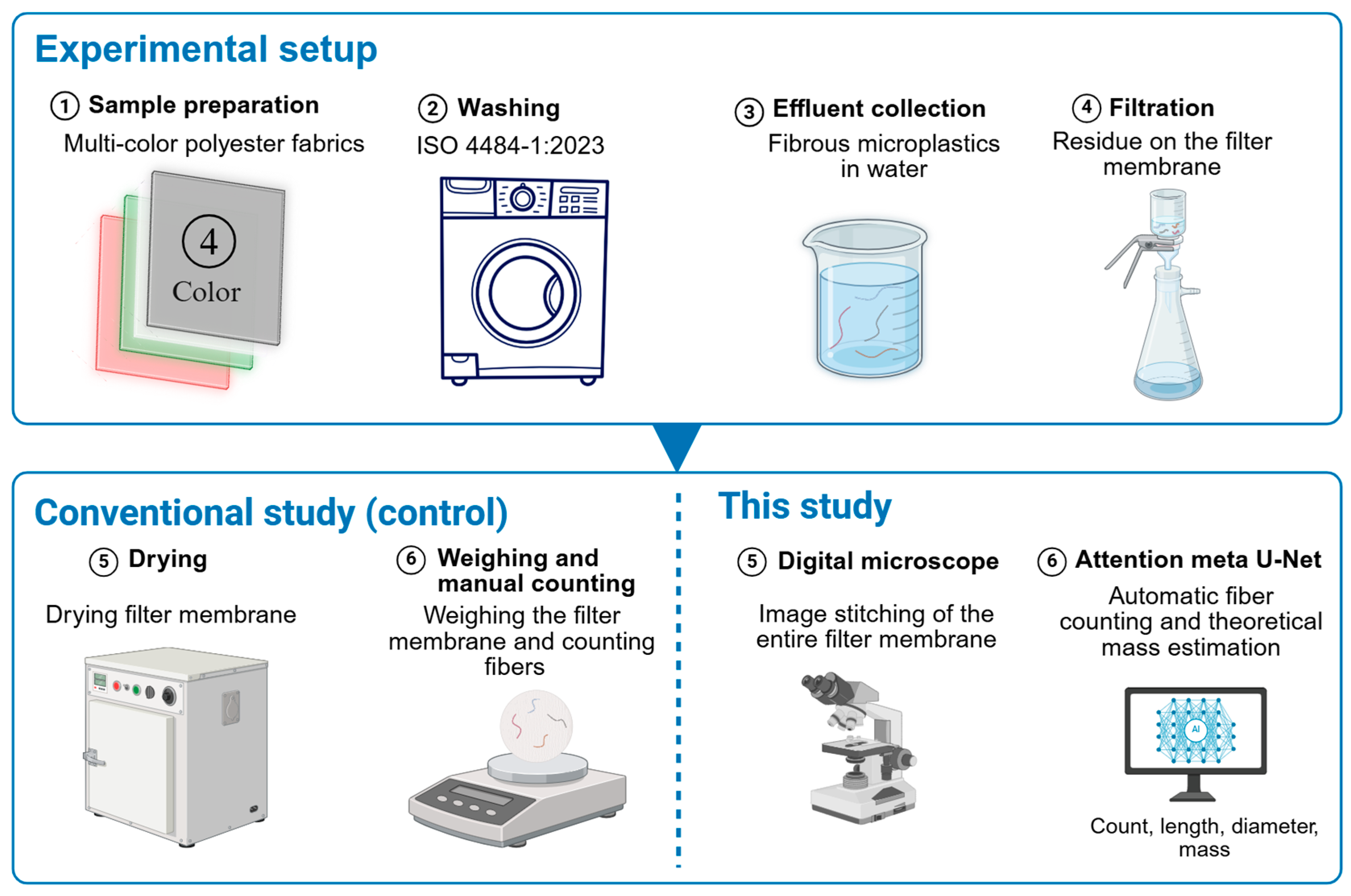
The fabric was prepared in accordance with ISO 4484-1:2023 [19]. Briefly, the fabric was initially cut into a rectangle measuring approximately 290 mm × 150 mm. Next, the edges were folded and secured using a 301-type stitch with polyester thread on a Bernina 1008 sewing machine (BERNINA International AG, Steckborn, Switzerland) to prevent fraying. The ISO standard specifies the use of a mechanical device capable of rotating samples at approximately 40 rpm, while maintaining precise temperature control throughout the process. In our study, this requirement was met by using a Datacolor Ahiba IR Pro (Datacolor, NJ, USA) laboratory dyeing machine. The fabrics were washed using DI water as follows. Each sample was immersed in 360 mL of DI water in a beaker with 50 stainless steel balls, each 6 mm in diameter. The beakers were mounted in the rotating holder, and the washing protocol was run at 40 °C for 45 min with continuous rotation at 40 rpm in the xy plane. The rotation of the holder results in the containers being inverted twice every rotation. After completion, the liquid was collected from each beaker and placed in glass bottles for subsequent study. The beaker was then rinsed three times with DI water to collect any remaining fiber fragments. To simulate real-life washing conditions involving multi-colored fabrics, the liquors collected from separate processing of differently colored fabrics were combined and subsequently filtered for further analysis. The experimental setup, including sample preparation, washing, filtration, imaging, and AIA of shed FMPs using the meta U-Net method, is shown in Figure 1.

Figure 1. Schematic overview of the experimental setup, including four color-variant synthetic fabrics, standardized washing protocol, effluent collection, and filtration. Additionally, conventional methods include drying, weighing, and manual counting. In contrast, this study proposes digital microscopy with stitched imaging and an automated fiber-counting method based on the attention meta U-Net.

2.3. Filtration, Imaging, and Characterization

Polyethersulfone (PES) membranes were used (47 mm; 0.22 µm). The filter membrane’s dry mass was determined using an electronic balance. The vacuum filtration device was prepared by placing a new filter membrane on the holder using tweezers, securing the funnel, and activating the vacuum. The liquor was carefully poured from the container onto the filter membrane, avoiding splashes. The sample container was rinsed three times, and all rinse water was poured into the filtration device. The filter membrane was collected, placed in an oven for 4 h at 50 °C, and then used to determine shedding mass using GA. GA for FMPs quantification involves physically separating and weighing particles to determine their total mass concentration (e.g., mg/L or mg/kg) in a sample. The supernatant and residual FMPs were isolated by filtering the samples onto a pre-weighed membrane, drying the membrane to a constant weight, and determining the microplastic mass from the resulting weight difference [36]. A separate membrane was used to filter the water containing FMPs for each of the PB, PW, PR, and PG fabrics to quantify fiber release, enabling shedding to be assessed independently for each color. For the multi-color analysis, the wash waters from each fabric type were combined and subsequently filtered through a separate membrane to enable integrated assessment of fiber shedding across all colors.

The filter membranes were analyzed with a Keyence digital microscope (Keyence, VHX-S650E, Keyence Corporation, Osaka, Japan). To obtain a high-resolution stitched image of a 47 mm filter membrane, approximately 600 individual images were acquired and computationally stitched using the Keyence microscope. A stitched image with a final resolution of 17,549 × 17,749 pixels was generated for analysis, corresponding to a spatial resolution of 2.17 µm/pixel. All images were captured under consistent acquisition settings, using the same illumination across all samples. Following image acquisition, post-processing was performed in Adobe Photoshop to remove non-essential peripheral regions of the membrane.

The mass conversion method used in this work is based on that by Hegarty et al. [31]. Briefly, assuming a cylindrical geometry, the mass of an individual fiber in mg ($M_i$) can be derived from its length, provided the polymer density ($\rho$) in mg/μm³ is known, D is the diameter, and $l_i$ is the length of the fiber as expressed in the following equation:

$$M_i=\rho \times {\displaystyle \frac{\pi }{4}}\times D^2\times l_i$$

(1)

A density of 1.38 g/cm³ (1.38 × 10⁻⁹ mg/μm³) was used for polyester fibers, and their diameter and length were used to obtain theoretical mass.

2.4. Architecture for Fibrous Microplastics Analysis Using Attention Meta U-Net

The attention-based meta U-Net was employed to overcome the limitations of conventional segmentation models in capturing the complex, elongated morphology and heterogeneity of FMPs. By integrating attention mechanisms with meta-feature learning, the model adaptively emphasizes relevant fiber structures while incorporating global statistical context from RGB distributions. This hybrid design represents a novel approach that enhances segmentation accuracy and robustness across varying imaging conditions, enabling more reliable quantitative characterization of FMPs. Figure S2, which outlines the processing pipeline, from image acquisition to quantitative fiber characterization, is structured into modular components with 3D-rendered elements that highlight hierarchical interdependencies.

The pipeline starts with the input image module, which processes original RGB images of dimensions H × W × 3. This input simultaneously feeds into two parallel pathways: the encoder path and the meta-feature extraction path. The encoder progressively downsamples the feature using four convolutional blocks with increasing channel depths [64, 128, 256, 512], with max pooling for spatial reduction. Concurrently, the meta-features module computes statistical properties, including the means (µR, µG, µB) and standard deviations (σR, σG, σB) of RGB channels, capturing essential image characteristics.

These meta-features are fed into a meta-learner, implemented as a fully connected (FC) neural network, where each FC layer (a dense layer performing linear transformations) is followed by a rectified linear unit (ReLU) activation function. The sequence FC → ReLU → FC → ReLU → FC enables the network to generate adaptive modulation parameters. At the core, the bottleneck layer (1024 features) integrates encoder outputs with meta-learner modulations through bidirectional connections, enabling context-aware feature adaptation. This is complemented by attention blocks that implement the attention mechanism $\mathsf{\psi }(\mathrm{g},\mathrm{x})=\mathsf{\sigma }\left(\mathsf{\psi }\mathrm{T}\right(\mathrm{R}\mathrm{e}\mathrm{L}\mathrm{U}(\mathrm{W}\mathrm{g}\mathrm{g}+\mathrm{W}\mathrm{x}\mathrm{x})\left)\right)$, selectively amplifying relevant features while suppressing noise. The decoder path employs transposed convolutions for up-sampling, incorporating attention-modulated skip connections to preserve spatial details. This leads to the output layer, which applies a 1 × 1, convolution with sigmoid activation to generate precise segmentation masks. Subsequent post-processing operations, including thresholding, morphological operations, and watershed segmentation, refine these masks into clean fiber representations. Feature extraction then quantifies fiber properties through skeletonization, and region props analysis, computing length, diameter, and area measurements.

Downstream components include visualization modules that generate diagnostic plots and 3D renderings, as well as performance metrics evaluation using accuracy, precision, and recall. The data-flow component encompasses the full pipeline from image input to analytical output. The supporting infrastructure includes parameter-optimization training, model-comparison benchmarking against standard U-Net and FCN architectures, and implementation details outlining the integration of PyTorch 2.11.0, CUDA 13.0, and OpenCV 4.13.0.

Annotations group components (Figure S2) into functional categories: Image Processing Pipeline, Feature Extraction and Enhancement, Meta-Learning Adaptation, Attention Mechanism, Reconstruction and Upsampling, Fiber Analysis and Measurement, Model Training and Optimization, and Performance Evaluation. Directional arrows indicate data flow relationships, with distinct colors highlighting meta-learning, attention, and primary processing connections. This visualization effectively communicates both the technical complexity and systematic workflow of an advanced computer vision system designed for high-precision fiber characterization and measurement.

2.5. Image Pre-Processing and Post-Processing

Each image underwent a standardized preprocessing pipeline to ensure compatibility with the deep learning model. The images were resized to a fixed width of 1920 pixels while maintaining their original aspect ratio, resulting in approximately 1920 × 1920-pixel dimensions. Pixel values were normalized to the range [0, 1] using the following equation:

$$I_{norm}={\displaystyle \frac{I_{raw}}{255}}$$

(2)

where I_raw is the original image, and I_norm is the normalized image. The normalized images were converted to PyTorch tensors with dimensions [batch, channels, height, width] and transferred to a GPU (CUDA) when available for accelerated processing. Additionally, meta-features were extracted from each image as the mean (μ) and standard deviation (σ) of each RGB channel, concatenated into a 6-dimensional vector mentioned in the equation below:

m = [μR, μG, μB, σR, σG, σB]

(3)

These meta-features were used by the meta-learning module to adaptively modulate the network’s feature representation based on image statistics.

Following the model prediction, the output segmentation mask underwent several preprocessing steps to extract individual fiber properties. The raw probability mask P ∈ [0, 1] was thresholded at T = 0.3 to generate a binary mask, as shown in the equation below:

$$B\left(x,y\right)=\left\{\begin{array}{cc}1\hfill & \hfill \mathrm{If} P\left(x,y\right)\ge T\\ 0\hfill & \hfill \mathrm{otherwise}\end{array}\right.$$

(4)

To exclude non-fiber artifacts, the original image was converted to the HSV color space, and a mask was applied to retain only non-black regions using the HSV range: hue ∈ [0, 179], saturation ∈ [40, 255], value ∈ [40, 255]. Morphological operations were performed to clean the binary mask, followed by a distance transformation, as shown in the equation below:

$$D(x,y)=\underset{\left(x^{\prime },y^{\prime }\right)\in \partial B}{\min }\sqrt{{(x-x^{\prime })}^2+{(y-y^{\prime })}^2}$$

(5)

where ∂B represents the boundary of the binary mask. Peak local maxima detection was used to initialize markers for the watershed algorithm, which separated overlapping fibers into individual instances. Each segmented fiber region was skeletonized to extract length measurements, while the equivalent diameter $D_{eq}$ was calculated from the area A, as mentioned in the equation below:

$$D_{eq}=2\sqrt{{\displaystyle \frac{A}{\pi }}}$$

(6)

To establish a robust benchmark for validation, manual quantification was performed by directly annotating and enumerating individual fibers on the stitched images using an Apple iPad and Pencil. Figure S3 illustrates the manual enumeration and labeling of fibers shed from PW fabrics across the membrane, which is used for validation. This comparison highlights the significant efficiency of the proposed AIA method: while manual counting is labor-intensive, the AIA system analyzes the equivalent membrane area in approximately 45 s.

3. Results and Discussion

3.1. Detection, Labeling, and Quantitative Analysis of Target-Colored Fibers

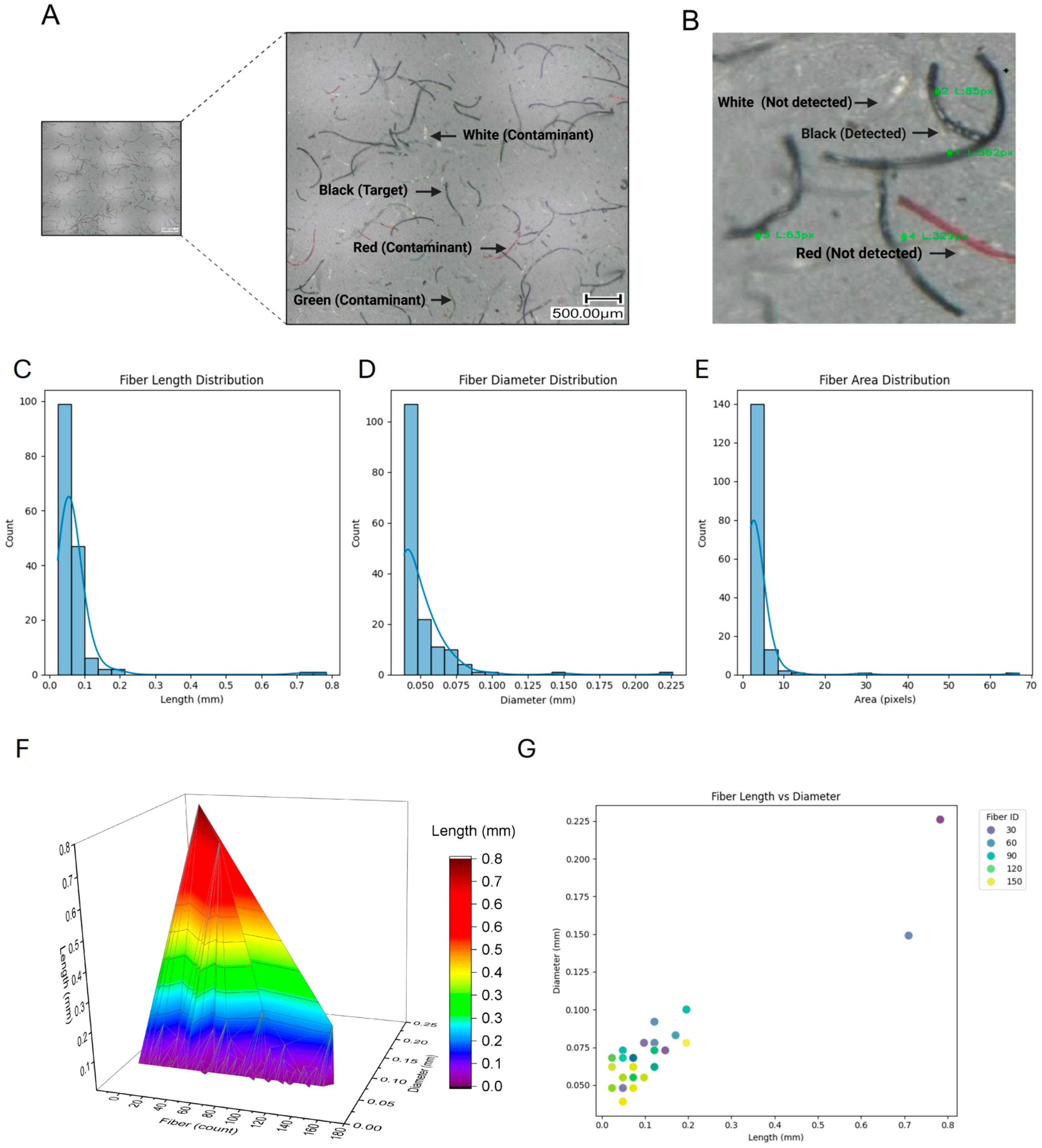
Image processing approaches have advanced markedly with improvements in computational power and algorithm design, offering substantial potential for characterizing laundry-derived FMPs. The AIA system employed in this study was used to identify and characterize both single-color and multi-color FMPs, enabling their analysis either independently or in combination. Although these AIA workflows differ in implementation, they generally follow a common sequence of analytical steps, beginning with the acquisition of images of the separate membranes. Our developed model detected and labeled 158 black fibers in the image of the filter membrane after washing with PB fabric (Figure 2). The pixel-based measurements revealed that most fibers were relatively small, with lengths ranging from 1 to 39 pixels and areas from 2 to 57 pixels, indicating the model’s ability to identify fine, elongated fibrous structures at high resolution. Spatial distribution analysis revealed that fibers were evenly dispersed throughout the entire image field, with centroid coordinates spanning x-values from 0 to 1918 and y-values from 0 to 1939. This comprehensive coverage suggests effective detection across different regions without significant spatial bias, which yields a visual appearance on the membrane comparable to what would be observed macroscopically with the unaided eye. Notably, the model identified both isolated fibers and clustered formations, maintaining accurate segmentation even in dense regions. The results highlight the model’s precision in measuring fiber dimensions, with consistent diameter measurements and accurate length estimates derived from skeletonization.

Figure 2. Integrated image analysis workflow and morphological characterization of fibrous microplastic (FMP) shedding from PB fabric. (A) Distinction between target (black) and non-target (white, green, red) FMPs based on their morphological characteristics within a magnified region. (B) Isolated detection of target FMPs following background subtraction and removal of non-target entities. (C) Distribution of fiber lengths shed from PB fabric samples. (D) Diameter profile of segmented FMPs. (E) Pixel-based area distribution of individual fibers quantified via image analysis. (F) Three-dimensional visualization of all segmented fibers, highlighting the overall length and diameter of the shed FMPs. (G) Scatter plot of fiber length-to-diameter distributions, with Fiber ID labels (30, 60, 90, 120, 150) representing groups of fibers exhibiting similar aspect ratios to facilitate comparative analysis.

Figure 2A,B illustrates the model’s discriminatory performance, demonstrating its ability to selectively and automatically detect the target color while effectively distinguishing it from contaminant fibers. Figure 2C–E illustrates the distributions of fiber length, diameter, and area by pixel, which are essential parameters for understanding fiber shedding behavior. Black FMPs with lengths ranging from approximately 0.024 mm to 0.783 mm and diameters between approximately 28 µm and 226 µm (Figure 2C,D) were analyzed. A minimum detectable fiber diameter of 28 µm was established and validated by manual annotation in ImageJ 1.51j8 software.

The integration of attention mechanisms and meta-learning modules enabled robust segmentation and quantification, even under variable imaging conditions. Figure 2F provides a comprehensive analysis of the shed black fibers, illustrating their overall morphological characteristics in a three-dimensional view. This 3D representation enables a more detailed evaluation of fiber geometry and spatial distribution. It represents the construction by mapping each detected fiber to a three-axis coordinate system, where the x-axis corresponds to fiber count, the y-axis to fiber length, and the z-axis to fiber diameter. Each point in the plot, therefore, reflects a single fiber, positioned according to its measured geometric attributes. By plotting all fibers simultaneously in this three-dimensional space, the graph visualizes the distribution of length and diameter across the entire sample. Additionally, the fiber length-to-diameter ratio is shown in Figure 2G. The length-to-diameter ratio is a critical geometric parameter that affects fiber fragmentation rates, providing valuable insight into their shedding behavior and eventual environmental fate.

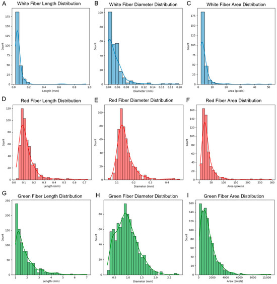
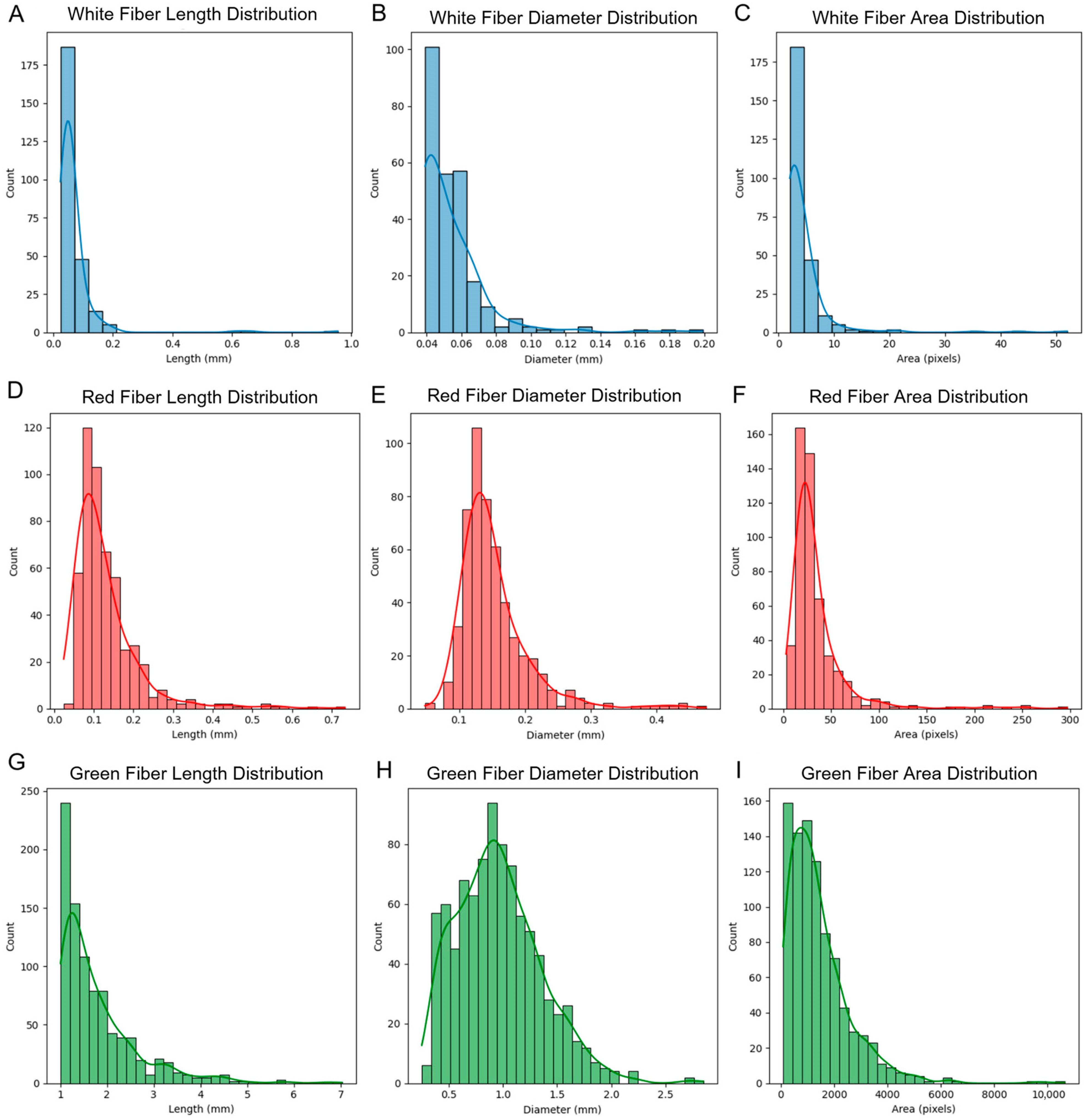
Similarly, the quantification of FMPs shed from PW, PR, and PG fabrics was performed separately using targeted color-based analysis, with FMPs classified by color (e.g., white, red, and green). A total of 257 white-colored fibers were detected using AIA across the filter membrane during the analysis of PW fabric shedding kinetics (Figure 3A–C), revealing substantial variation in morphological dimensions when analyzing the membrane used to filter the wash water from PW fabric. In contrast, the manual method detected 263 FMPs, which were used as the reference for validation. The AIA achieved approximately 98% accuracy relative to this benchmark. Length measurements spanned from 24 µm to 955 µm, reflecting a broad distribution of longitudinal fiber extension (Figure 3A). The fiber diameters ranged from 39 µm to 199 µm, indicating heterogeneity in the cross-sectional structure (Figure 3B). These metrics suggest diverse fragmentation and deposition behavior, potentially influenced by washing or abrasion of the PW fabrics. White fibers present a measurement challenge because their transparent or semi-transparent nature causes them to appear grey under optical microscopy, reducing contrast and making automated detection less reliable. This low visual distinction increases the likelihood of misclassification or undercounting in image-analysis workflows, representing a notable limitation when quantifying mixed-color fiber samples.

Figure 3. Comparative morphological characterization of fibrous microplastics shed from different fabrics based on color-targeted analysis. (A–C) present the length distribution, diameter variation, and pixel-based area distribution of white fibers shed from PW fabric; (D–F) show the corresponding parameters for red fibers from PR fabric; and (G–I) illustrate the same metrics for green fibers from PG fabric.

In comparison, 514 red-colored shed fibers were identified in the PR fabric, with lengths ranging from 24 µm to 734 µm (Figure 3D) and diameters ranging from 48 µm to 476 µm (Figure 3E). The green-colored fiber population extracted from PG fabric consisted of 897 individual fibers, exhibiting notable variability in both length and diameter (Figure 3G–I). The pixel-level distribution reflects the overall variability in fiber detection, indicating whether fibers are consistent in size or exhibit a wide range of dimensions. This variability provides a general measure of the uniformity of fiber morphology for detecting fibers in the complex environmental sample. Figure 3C, Figure 3F, and Figure 3I illustrate the pixel area distributions for the detected white, red, and green fibers, respectively. The white fibers (Figure 3C) exhibit a notably narrower distribution profile compared to the red (Figure 3F) and green (Figure 3I) fibers. This indicates that the white fibers possess a significantly higher degree of morphological homogeneity than their red and green counterparts. This heterogeneity in the red and green fibers in the area distribution by pixel is likely due to pigment layering and subsequent color shedding, resulting in multiple fragmented deposits of green coloration across the membrane. The colored polyester fabrics used in this study were purchased as commercially dyed materials, and their polymeric composition was verified as 100% polyester using FTIR prior to the washing experiments to ensure the absence of mixed-blend or contaminant fibers. The use of color-specific fibers serves as a controlled system for evaluating the model’s ability to distinguish FMPs from non-plastic particles under mixed-color conditions. However, it remains unclear how to differentiate natural fibers from synthetic fibers using AIA.

3.2. Fiber Detection and Contaminant Exclusion Mechanisms, Including Overlapped Fibers

To enhance detection accuracy and minimize interference from non-target elements, fiber segmentation was performed on a cropped region of the original image, focusing on a localized area of interest. This approach excluded fibers of differing coloration and potential non-fibrous contaminants, thereby improving the precision of morphological analysis. The cropped region was processed using an attention U-Net architecture integrated with meta-learning, enabling high-fidelity detection even within structurally heterogeneous regions, as shown in Figure 4 and Figure S4.

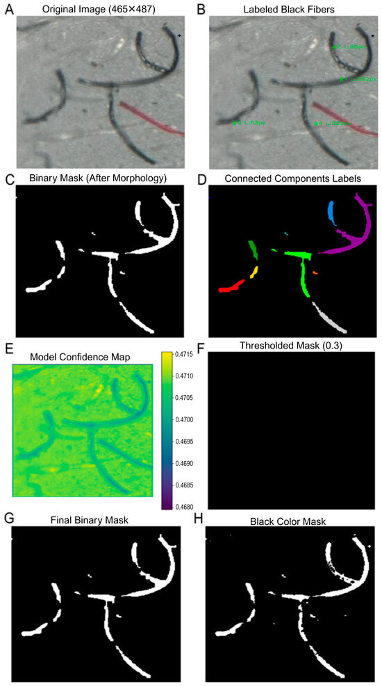
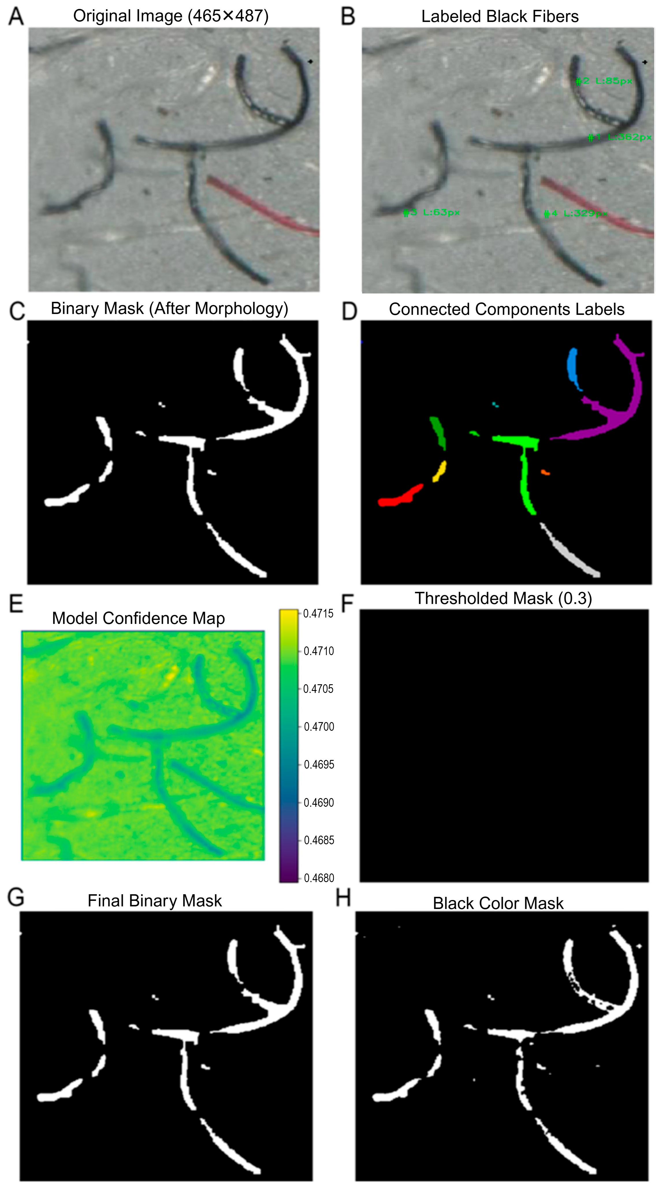
Figure 4. The stepwise progression of the black fiber detection pipeline, from the original image (A) through segmentation and refinement stages. Labeled fibers (B) are converted into a binary mask (C), followed by connected component analysis (D) to isolate individual structures. The model’s confidence map (E) guides thresholding (F), resulting in a post-processed output (G) and a final detection result (H) that accurately resolves black fiber regions within heterogeneous sample areas.

Attention blocks in the U-Net selectively enhance skip connection features, while the meta-learner modulates bottleneck features based on image statistics. This combination enhances the model’s sensitivity to subtle fiber patterns, enabling it to generalize across varying imaging conditions. Postprocessing with watershed segmentation, distance transforms, and skeletonization ensures accurate separation and quantification of individual fibers. Extracted fiber metrics, including length, diameter, area, and centroid position, form the basis for statistical analyses, scatter plots, and 3D visualizations.

Figure 4 illustrates the end-to-end fiber detection process, from the raw input image to refined segmentation of black fibers. The subplots are arranged sequentially, presenting each computational stage of the pipeline. The process begins with the original image (Figure 4A), which provides the contextual foundation for subsequent stages. This image typically contains a mixture of background textures, noise, and fibers of interest. Without preprocessing, the presence of these confounding elements would make direct fiber detection unreliable. Thus, the pipeline introduces a binary mask (Figure 4C) that isolates potential fiber regions. This mask is generated using intensity thresholding and morphological operations to suppress irrelevant background information and enhance fiber-like structures. Once the binary mask is created, a connected component analysis is performed to separate distinct fiber candidates (Figure 4D). This step is particularly important in scenarios where multiple fibers overlap or exist in close proximity. By assigning unique labels to connected regions, the algorithm ensures that each fiber is treated as an individual entity for downstream analysis. This labeled fiber representation enables quantitative measurements, such as length, orientation, and curvature, to be extracted per fiber. A key feature of this figure is the inclusion of the model confidence map. Unlike hard-thresholded outputs, the confidence map visualizes the probabilistic strength of detection across the image. Regions with higher values correspond to areas where the model is highly confident in detecting fibers (Figure 4E), while lower values indicate uncertainty. This provides interpretability and insight into model behavior, allowing researchers to identify ambiguous regions that may require further refinement. Following the confidence map, a thresholding operation is applied to remove low-confidence detections (Figure 4F). This results in a cleaner binary mask with reduced noise, ensuring that only highly probable fiber structures are retained. The pipeline culminates in the final mask, which accurately highlights black fibers (Figure 4H). Taken together, this stepwise pipeline demonstrates robustness and transparency, enabling reproducibility and facilitating error diagnosis.

3.3. Comprehensive Intensity-Based Analysis of Detected Fibers

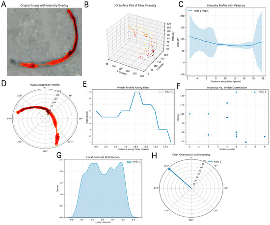
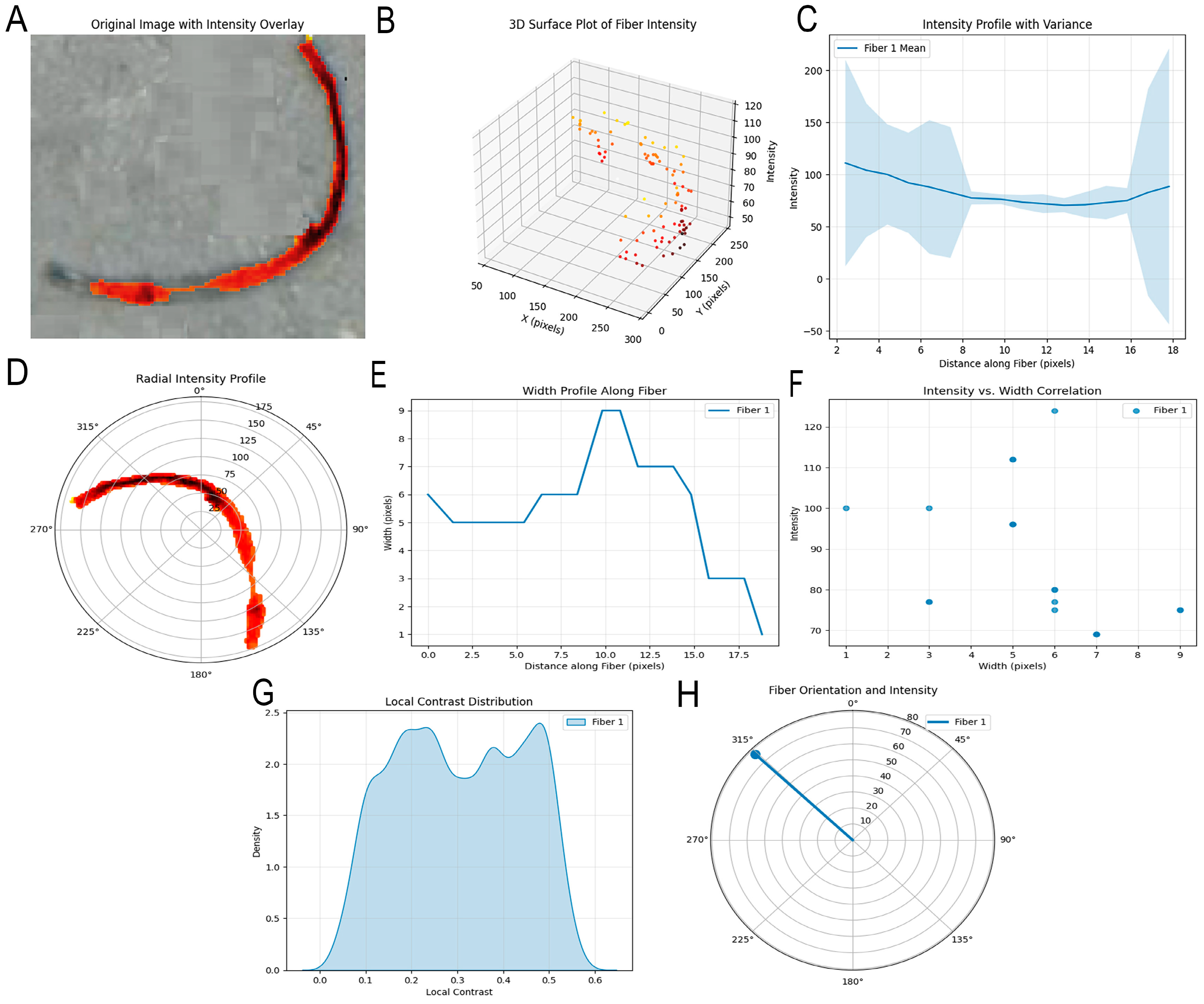
Figure 5 provides three complementary perspectives: intensity distribution, three-dimensional surface representation, and profile-based characterization. Figure 5A overlays intensity distributions onto the detected fibers within the original image. This combined visualization retains contextual information while simultaneously highlighting pixel-level brightness variations. Such overlays are crucial for distinguishing fibers with different material compositions, densities, or illumination conditions. Variations in intensity may reflect structural heterogeneity, surface roughness, or even fiber defects. Thus, intensity distribution analysis provides an additional layer of information beyond simple binary segmentation. The three-dimensional surface representation treats pixel intensities as topographical heights, as shown in Figure 5B. In this representation, brighter regions appear elevated, while darker areas recede, resulting in a landscape-like visualization of the fiber structure. This approach provides insights into thickness variations and overlapping fibers, which can be challenging to discern in two-dimensional projections. Figure 5C focuses on profile-based characterization, in which intensity values are plotted along the trajectories of selected fibers. These profiles capture local brightness fluctuations, enabling micro-level analysis of fiber consistency. To further characterize the optical and geometric properties of individual fibers, several quantitative image-derived features were extracted (Figure 5D–H). The radial intensity profile (Figure 5D) captures angular variations in local pixel intensity, providing insight into circumferential heterogeneity associated with dye distribution and surface reflectance. The longitudinal intensity profile (Figure 5E) quantifies signal variation along the fiber axis, while the intensity–width relationship (Figure 5F) evaluates whether local geometric changes influence measured optical response. The distribution of local contrast values (Figure 5G) summarizes edge sharpness and textural variability across the fiber field and serves as an indicator of segmentation reliability. Finally, the orientation-intensity representation (Figure 5H) identifies the dominant alignment direction of each fiber and its associated signal magnitude, revealing directional patterns and structural heterogeneity within the sample. A regular, stable profile suggests uniform structural properties, while irregular fluctuations may indicate defects, surface contamination, or inconsistencies in fiber formation. By examining multiple profiles, it is possible to identify patterns of variation across the dataset, making this approach highly valuable for both research and industrial monitoring.

Figure 5. Represents a comprehensive analysis of detected fibers, emphasizing both structural and intensity-based features. (A) displays the original input image with intensity overlay; (B) 3D surface plot with fiber intensity. The intensity distribution across fibers is shown in (C), followed by a radial intensity profile in (D), which captures local intensity gradients. (E) Illustrates the intensity profile along selected fiber axes, and (F) highlights the correlation between intensity and width. (G) depicts the local contrast distribution across the fiber field, and (H) presents fiber orientation and corresponding intensity, revealing directional patterns and signal heterogeneity within the sample.

Together, Figure 4 and Figure 5 provide a holistic narrative of the fiber detection and analysis process. Figure 4 highlights each intermediate stage of the pipeline, enabling a clear understanding of how raw data are transformed into meaningful fiber representations. This stepwise breakdown enhances interpretability and supports reproducibility, as researchers can replicate or refine individual stages according to their specific requirements. In contrast, Figure 5 shifts the focus to analytical depth.

By leveraging intensity profile, surface plots, and profile-based characterizations, Figure 5C illustrates the set of evaluations that can be performed once reliable segmentation is achieved. In textile manufacturing, for example, the ability to detect black, red, white, or green fibers and analyze their intensity distributions could facilitate automated detection of the shed FMPs from textile wastewater. Deviations in intensity or irregularities in fiber profiles may reveal defects such as weak spots, contamination, or weaving inconsistencies, which could help understand the fiber’s mechanical properties.

3.4. Multi-Colored Fiber Analysis

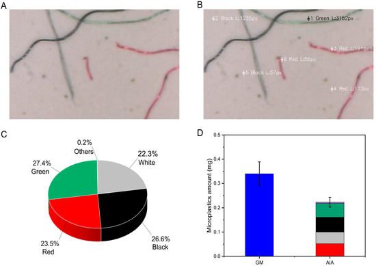
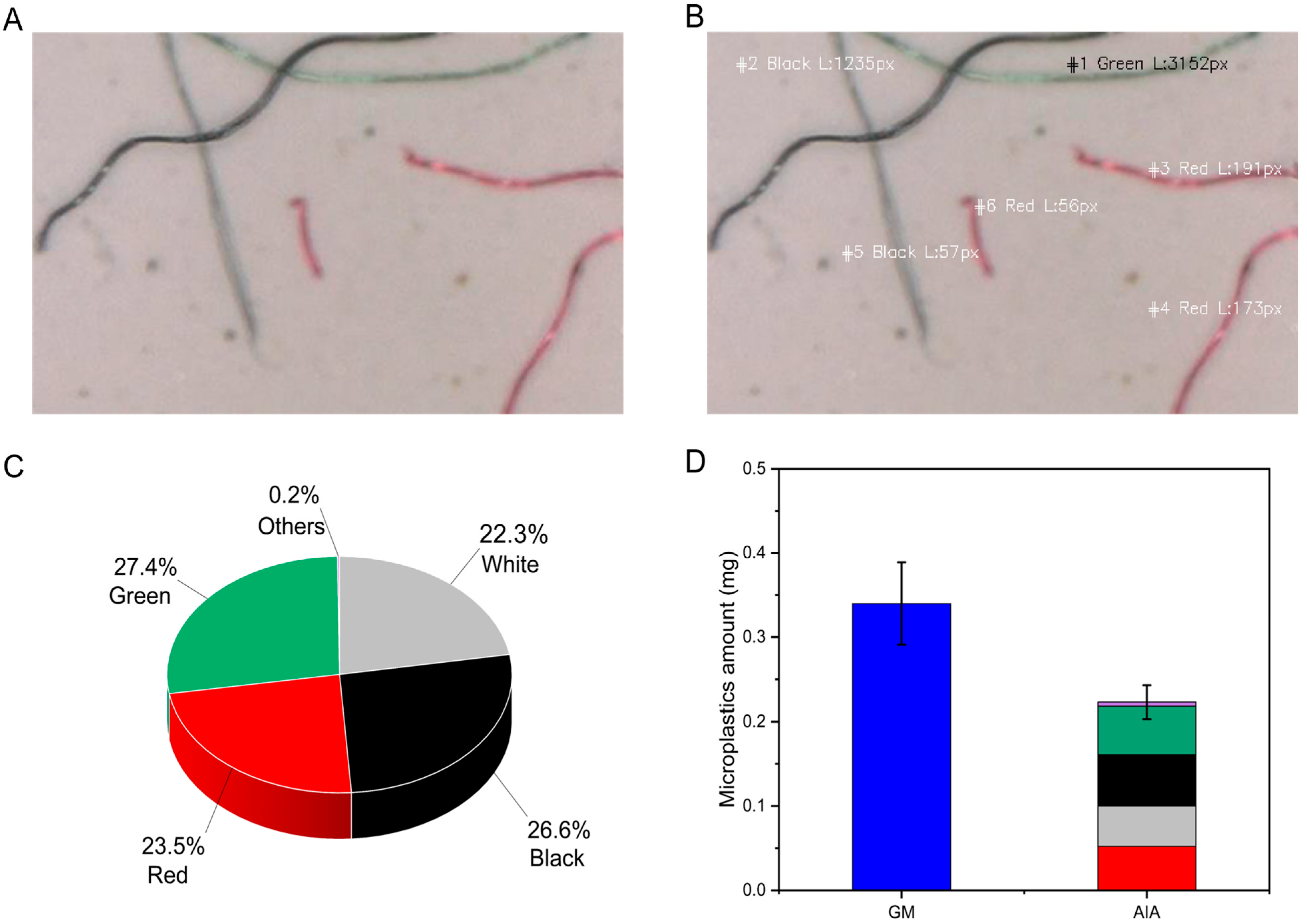
To better replicate real-world shedding conditions, where environmental samples typically contain fibers from multiple colors, we prepared a complex mixture by combining effluents from different colored textiles and subsequently filtering them. This approach allowed us to generate a representative heterogeneous sample. The tested AIA method detects and differentiates fibers of various colors, as demonstrated in Figure 6. Figure 6A shows the original unlabeled image of a magnified region, while Figure 6B presents the AIA-processed and labeled output. The analyzed sample was reported by the AIA system to contain white (22.3%), black (26.6%), red (23.5%), green (27.4%), and other colors (0.2%) based on the number of detections (Figure 6C). Fiber-like particles exhibiting colors not included in the predefined categories were classified as ‘other’. These results confirm that the AIA method can recognize and classify fibers across a broad range of colors in complex, environmentally relevant samples. A limitation of the system is its reduced ability to classify fibers with colors outside the predefined categories, as these undefined hues introduce uncertainty into the analysis. Future refinements to the color-classification framework could improve performance for these additional color groups. Relative to GM, the AIA consistently yielded lower mass values for FMPs. This discrepancy arises because GM captures the total weight of all retained material, including moisture, mineral residues, and non-fibrous contaminants. The shed mass from the mixed fibers in a filter membrane was determined by GM and 0.34 ± 0.049 mg. In comparison, AIA quantified the theoretical mass of shed red, white, black, and green colors at approximately 0.052 mg, 0.048 mg, 0.061 mg, and 0.057 mg, respectively, with a standard deviation of 0.02, as shown in Figure 6D. Although the theoretical mass-estimation approach is influenced by both the number of fibers detected and the accuracy of the underlying model, the proposed framework offers a foundational basis for estimating the mass of shed fibers and provides a platform for further methodological refinement. Results from the AIA enable more precise measurement due to its volume-to-density calculation of the target materials. In contrast, the GM primarily relies on bulk weighing of the shed FMPs, which may overlook small fractions of shed FMPs, sample loss during handling, or environmental moisture absorption by the materials or the filter membrane.

Figure 6. AIA-based detection and color classification of mixed fibrous microplastics (FMPs) samples. (A) Original unlabeled image of the mixed-color FMPs sample. (B) AIA-labeled image showing automated identification; (C) detection based on fiber colors, including white (22.3%), black (26.6%), red (23.5%), green (27.4%), and others (0.2%), and (D) comparison of the shedding amount by the GM and AIA method, the red, white, black, green markers denoting their respective fiber categories, and purple indicating other fibers.

Although drying the filter membrane before and after measurement is intended to minimize moisture interference, immediate exposure to ambient air following oven dry can lead to rapid moisture reabsorption, potentially exacerbating the issue.

3.5. Performance Comparison, Environmental Impact, and Limitations

A comparative evaluation of existing approaches for FMP quantification shows substantial progress but also persistent limitations in automated analysis. Early image-processing methods, including threshold-based segmentation with contour and junction detection, achieved a high binary accuracy of approximately 95% yet struggled with complex morphologies and overlapping fibers [31]. Tools such as TUM-ParticleTyper performed comparably to expert analysis but showed reduced reliability in agglomerated or densely entangled samples [37].

Deep learning methods, especially U-Net–based models, have improved fiber detection compared to earlier techniques. Some enhanced versions achieved good overall accuracy and balanced performance [33], while more advanced combined approaches reported very high results but required more complex workflows and large amounts of training data [38]. Other models also performed well but showed limitations in consistently detecting fibers under different imaging conditions [39]. Methods specifically designed to separate tangled fibers improved this aspect, but their overall detection accuracy remained relatively low, particularly in dense and overlapping fiber networks [40,41]. In contrast, the proposed attention-based U-Net integrated with meta-learning achieves high accuracy (up to 98%) compared to manual counting. The incorporation of attention mechanisms and meta-feature–driven adaptation enhances the model’s ability to handle variations in intensity, color, and overlapping structures, challenges that previous methods do not fully address. These results demonstrate the improved accuracy and generalization capability of the proposed framework for reliable FMP quantification.

In addition, the environmental significance of this work lies in enabling accurate and scalable quantification of FMPs, which is critical for assessing textile-derived pollution. Current monitoring methods are often slow and inconsistent, limiting reliable estimation of MP emissions from domestic laundering. The proposed framework allows rapid, high-accuracy analysis, improving standardization and reproducibility. This supports more reliable evaluation of mitigation strategies and strengthens data-driven environmental monitoring and management.

The current framework has limitations: it cannot provide chemical spectral information or identify different polymer types, as pixel-based image analysis does not capture the molecular signatures required for chemical discrimination. Although the model can successfully separate overlapping fibers, including multi-color overlaps, it inevitably loses spatial detail at the intersection regions due to occlusion. Future integration of multispectral or hyperspectral imaging could enable polymer-specific spectral characterization and overcome these limitations in chemical identification, even for the colorless fibers.

4. Conclusions

This study introduces an automated framework for quantifying FMPs released during textile washing, offering a substantial improvement over existing analytical methods. By applying the model to full-membrane stitched images, we demonstrate reliable detection, segmentation, and characterization of fibers across a wide range of colors and morphologies. The system accurately identified fibers with multiple colors and distinguished target-color fibers within mixed-color samples, even when overlapping, highlighting its robustness under realistic conditions. These results show that automated analysis can replace labor-intensive manual counting, reducing processing time from hours to approximately 45 s per filter membrane while maintaining high accuracy.

Beyond count accuracy, the framework provides consistent geometric and mass estimates without the moisture sensitivity or false-positive issues associated with gravimetric methods. The ability to analyze entire filter membranes eliminates sampling bias and enhances reproducibility, supporting more standardized and scalable monitoring of textile-derived FMP pollution. Although the model cannot yet recover structural information at fiber intersections or differentiate natural from synthetic fibers, these limitations point to clear directions for future development, including real-time monitoring and integration with material-specific classifiers. Overall, the approach establishes a strong foundation for next-generation, high-throughput environmental MP analysis.

References

- Thompson, R.C.; Olsen, Y.; Mitchell, R.P.; Davis, A.; Rowland, S.J.; John, A.W.; McGonigle, D.; Russell, A.E. Lost at sea: Where is all the plastic? Science 2004, 304, 838. [Google Scholar] [CrossRef] [PubMed]
- Frias, J.; Nash, R. Microplastics: Finding a consensus on the definition. Mar. Pollut. Bull. 2019, 138, 145–147. [Google Scholar] [CrossRef]
- Hartmann, N.B.; Huffer, T.; Thompson, R.C.; Hassellov, M.; Verschoor, A.; Daugaard, A.E.; Rist, S.; Karlsson, T.; Brennholt, N.; Cole, M.; et al. Are We Speaking the Same Language? Recommendations for a Definition and Categorization Framework for Plastic Debris. Environ. Sci. Technol. 2019, 53, 1039–1047. [Google Scholar] [CrossRef]
- Arthur, C.; Baker, J.E.; Bamford, H.A. Proceedings of the International Research Workshop on the Occurrence, Effects and Fate of Microplastic Marine Debris, Tacoma, WA, USA, 9–11 September 2008; National Oceanic and Atmospheric Administration: Silver Spring, MD, USA, 2009.
- Ryan, P.G. A Brief History of Marine Litter Research. In Marine Anthropogenic Litter; Bergmann, M., Gutow, L., Klages, M., Eds.; Springer International Publishing: Cham, Switzerland, 2015; pp. 1–25. [Google Scholar]
- Iyare, P.U.; Ouki, S.K.; Bond, T. Microplastics removal in wastewater treatment plants: A critical review. Environ. Sci. Water Res. Technol. 2020, 6, 2664–2675. [Google Scholar] [CrossRef]
- Ni, N.; Qiu, J.; Ge, W.; Guo, X.; Zhu, D.; Wang, N.; Luo, Y. Fibrous and Fragmented Microplastics Discharged from Sewage Amplify Health Risks Associated with Antibiotic Resistance Genes in Aquatic Environments. Environ. Sci. Technol. 2025, 59, 15919–15930. [Google Scholar] [CrossRef]
- Ma, C.; Shi, H.; Slaveykova, V.I. Entanglement of Daphnia magna by Fibrous Microplastics through “Hook and Loop” Action. Environ. Sci. Technol. Lett. 2024, 11, 433–437. [Google Scholar] [CrossRef]
- Kawecki, D.; Nowack, B. Polymer-Specific Modeling of the Environmental Emissions of Seven Commodity Plastics As Macro- and Microplastics. Environ. Sci. Technol. 2019, 53, 9664–9676. [Google Scholar] [CrossRef]
- Zhang, Y.; Haque, A.N.M.A.; Ranjbar, S.; Tester, D.; Naebe, M. A Standard Terminology for the Description of Fibrous Microplastics from Textiles. Adv. Sci. Technol. 2024, 146, 33–36. [Google Scholar] [CrossRef]
- Thompson, R.C.; Courtene-Jones, W.; Boucher, J.; Pahl, S.; Raubenheimer, K.; Koelmans, A.A. Twenty years of microplastic pollution research-what have we learned? Science 2024, 386, eadl2746. [Google Scholar] [CrossRef]
- Napper, I.E.; Thompson, R.C. Release of synthetic microplastic plastic fibres from domestic washing machines: Effects of fabric type and washing conditions. Mar. Pollut. Bull. 2016, 112, 39–45. [Google Scholar] [CrossRef] [PubMed]
- Cai, Y.; Yang, T.; Mitrano, D.M.; Heuberger, M.; Hufenus, R.; Nowack, B. Systematic Study of Microplastic Fiber Release from 12 Different Polyester Textiles during Washing. Environ. Sci. Technol. 2020, 54, 4847–4855. [Google Scholar] [CrossRef]
- Rathinamoorthy, R.; Raja Balasaraswathi, S. (Eds.) Domestic Laundry—A Major Cause of Microfiber Shedding. In Microfiber Pollution; Springer Nature Singapore: Singapore, 2022; pp. 107–149. [Google Scholar]
- Pinlova, B.; Hufenus, R.; Nowack, B. Systematic study of the presence of microplastic fibers during polyester yarn production. J. Clean. Prod. 2022, 363, 132247. [Google Scholar] [CrossRef]
- Jabbar, A.; Tausif, M. Investigation of ring, airjet and rotor spun yarn structures on the fragmented fibers (microplastics) released from polyester textiles during laundering. Text. Res. J. 2023, 93, 5017–5028. [Google Scholar] [CrossRef]
- Palacios-Marín, A.V.; Jabbar, A.; Tausif, M. Fragmented fiber pollution from common textile materials and structures during laundry. Text. Res. J. 2022, 92, 2265–2275. [Google Scholar] [CrossRef]
- Yang, T.; Luo, J.; Nowack, B. Characterization of Nanoplastics, Fibrils, and Microplastics Released during Washing and Abrasion of Polyester Textiles. Environ. Sci. Technol. 2021, 55, 15873–15881. [Google Scholar] [CrossRef]
- BS EN ISO 4484-4481:2023; Microplastics from Textile Sources—Part 1: Determination of Material Loss from Fabrics During Washing. British Standards Institution (BSI): London, UK, 2023.
- De Falco, F.; Di Pace, E.; Cocca, M.; Avella, M. The contribution of washing processes of synthetic clothes to microplastic pollution. Sci. Rep. 2019, 9, 6633. [Google Scholar] [CrossRef]
- De Falco, F.; Gentile, G.; Di Pace, E.; Avella, M.; Cocca, M. Quantification of microfibres released during washing of synthetic clothes in real conditions and at lab scale⋆. Eur. Phys. J. Plus 2018, 133, 257. [Google Scholar] [CrossRef]
- Wang, C.; Chen, W.; Zhao, H.; Tang, J.; Li, G.; Zhou, Q.; Sun, J.; Xing, B. Microplastic Fiber Release by Laundry: A Comparative Study of Hand-Washing and Machine-Washing. ACS ES T Water 2023, 3, 147–155. [Google Scholar] [CrossRef]
- Stanton, T.; Stanes, E.; Gwinnett, C.; Lei, X.; Cauilan-Cureg, M.; Ramos, M.; Sallach, J.B.; Harrison, E.; Osborne, A.; Sanders, C.H.; et al. Shedding off-the-grid: The role of garment manufacturing and textile care in global microfibre pollution. J. Clean. Prod. 2023, 428, 139391. [Google Scholar] [CrossRef]
- De Falco, F.; Cocca, M.; Avella, M.; Thompson, R.C. Microfiber Release to Water, Via Laundering, and to Air, via Everyday Use: A Comparison between Polyester Clothing with Differing Textile Parameters. Environ. Sci. Technol. 2020, 54, 3288–3296. [Google Scholar] [CrossRef] [PubMed]
- Haap, J.; Classen, E.; Beringer, J.; Mecheels, S.; Gutmann, J.S. Microplastic Fibers Released by Textile Laundry: A New Analytical Approach for the Determination of Fibers in Effluents. Water 2019, 11, 2088. [Google Scholar] [CrossRef]
- Kelly, M.R.; Lant, N.J.; Kurr, M.; Burgess, J.G. Importance of Water-Volume on the Release of Microplastic Fibers from Laundry. Environ. Sci. Technol. 2019, 53, 11735–11744. [Google Scholar] [CrossRef]
- Hyeon, Y.; Kim, S.; Ok, E.; Park, C. A fluid imaging flow cytometry for rapid characterization and realistic evaluation of microplastic fiber transport in ceramic membranes for laundry wastewater treatment. Chem. Eng. J. 2023, 454, 140028. [Google Scholar] [CrossRef]
- Elkhatib, D.; Oyanedel-Craver, V. A Critical Review of Extraction and Identification Methods of Microplastics in Wastewater and Drinking Water. Environ. Sci. Technol. 2020, 54, 7037–7049. [Google Scholar] [CrossRef]
- Tiffin, L.; Hazlehurst, A.; Sumner, M.; Taylor, M. Reliable quantification of microplastic release from the domestic laundry of textile fabrics. J. Text. Inst. 2021, 113, 558–566. [Google Scholar] [CrossRef]
- Murden, S.; Macintyre, L. Low-cost, high-throughput quantification of microplastics released from textile wash tests: Introducing the fibre fragmentation scale. Camb. Prism. Plast. 2024, 2, e30. [Google Scholar] [CrossRef]
- Hegarty, J.; dos Reis, R.; Dravid, V.P. Laundry to Laboratory: Automated Image Analysis for the Characterization of Fibrous Microplastics. ACS ES T Water 2024, 5, 2848–2860. [Google Scholar] [CrossRef]
- Lv, L.; Yan, X.; Feng, L.; Jiang, S.; Lu, Z.; Xie, H.; Sun, S.; Chen, J.; Li, C. Challenge for the detection of microplastics in the environment. Water Environ. Res. 2021, 93, 5–15. [Google Scholar] [CrossRef] [PubMed]
- Lee, K.S.; Chen, H.L.; Ng, Y.S.; Maul, T.; Gibbins, C.; Ting, K.-N.; Amer, M.; Camara, M. U-Net skip-connection architectures for the automated counting of microplastics. Neural Comput. Appl. 2022, 34, 7283–7297. [Google Scholar] [CrossRef]
- Nguyen, B.; Claveau-Mallet, D.; Hernandez, L.M.; Xu, E.G.; Farner, J.M.; Tufenkji, N. Separation and Analysis of Microplastics and Nanoplastics in Complex Environmental Samples. Acc. Chem. Res. 2019, 52, 858–866. [Google Scholar] [CrossRef]
- Amos, P.; Crumpton, W.G.; Wilkinson, G.; Milosevic, D.; Eads, D.; Jovanovic, B. Microplastics in 132 Iowa lakes and variability in relation to abiotic, biotic, and anthropogenic factors. Environ. Pollut. 2025, 369, 125839. [Google Scholar] [CrossRef] [PubMed]
- Hidalgo-Ruz, V.; Gutow, L.; Thompson, R.C.; Thiel, M. Microplastics in the marine environment: A review of the methods used for identification and quantification. Environ. Sci. Technol. 2012, 46, 3060–3075. [Google Scholar] [CrossRef]
- Von der Esch, E.; Kohles, A.J.; Anger, P.M.; Hoppe, R.; Niessner, R.; Elsner, M.; Ivleva, N.P. TUM-ParticleTyper: A detection and quantification tool for automated analysis of (Microplastic) particles and fibers. PLoS ONE 2020, 15, e0234766. [Google Scholar] [CrossRef] [PubMed]
- Hao, Y.; Wang, P.; Cui, M.; Zeng, Z.; Ma, S.; Li, Y.; Zou, T.; Fang, X.; Lin, L. Automatic localization and segmentation of adherent microplastics in optical micrographs based on improved YOLOv5 and adaptive perceptual UNET 3+++. Biomed. Signal Process. Control 2024, 95, 106399. [Google Scholar] [CrossRef]
- Lee, G.; Jung, J.; Moon, S.; Jung, J.; Jhang, K. Microscopic Image Dataset with Segmentation and Detection Labels for Microplastic Analysis in Sewage: Enhancing Research and Environmental Monitoring. Microplastics 2024, 3, 264–275. [Google Scholar] [CrossRef]
- Wegmayr, V.; Sahin, A.; Sæmundsson, B.; Buhmann, J.M. Instance Segmentation for the Quantification of Microplastic Fiber Images. In Proceedings of the 2020 IEEE Winter Conference on Applications of Computer Vision (WACV), Snowmass Village, CO, USA, 1–5 March 2020; pp. 2199–2206. [Google Scholar]
- Xu, J.; Wang, Z. Intelligent classification and pollution characteristics analysis of microplastics in urban surface waters using YNet. J. Hazard. Mater. 2024, 467, 133694. [Google Scholar] [CrossRef] [PubMed]
Disclaimer/Publisher’s Note: The statements, opinions and data contained in all publications are solely those of the individual author(s) and contributor(s) and not of MDPI and/or the editor(s). MDPI and/or the editor(s) disclaim responsibility for any injury to people or property resulting from any ideas, methods, instructions or products referred to in the content. |
© 2026 by the authors. Licensee MDPI, Basel, Switzerland. This article is an open access article distributed under the terms and conditions of the Creative Commons Attribution (CC BY) license.